Convolutional Neural Network#
from sklearn.datasets import fetch_openml
from sklearn.model_selection import train_test_split
import numpy as np
import matplotlib.pyplot as plt
from scipy.signal import convolve2d
This Jupyter Notebook showcases the implementation of a simple Convolutional Neural Network (CNN) for image classification. The notebook includes the definition of the CNN architecture.
We apply the network on the famous mnist dataset. The dataset contains images depicting handwritten numbers. The numbers range from zero to nine. The goal is to correctly predict the number shown on the image.
mnist = fetch_openml('mnist_784', as_frame=False)
X_train, X_test, y_train, y_test = train_test_split(mnist.data, mnist.target, test_size=0.2, random_state=42)
X_train = X_train.reshape(-1, 28, 28) / 255
X_test = X_test.reshape(-1, 28, 28) / 255
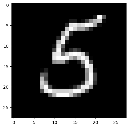
plt.imshow(X_train[0], cmap='gray')
print('Shape:', X_train[0].shape)
print('Label:', y_train[0])
Shape: (28, 28)
Label: 5
Convolution Refresher#
In the context of image processing, convolution is commonly used for tasks such as blurring, edge detection, and feature extraction. It involves sliding a small matrix called a kernel, filter or mask over an image and performing a mathematical operation at each position. The result of this operation is a new image that highlights certain features or characteristics of the original image. Let’s look at an example.
kernels = []

# Sharpening Filter
kernel = (-1 * np.ones((3,3)))
kernel[1,1] = 9
kernels.append(kernel.copy())

# Horizontal Edge Detector
kernel = np.zeros((3,3))
kernel[0, :] = 1
kernel[2, :] = -1
kernels.append(kernel.copy())

# Vertical Edge Detector
kernel = np.zeros((3,3))
kernel[:, 0] = 1
kernel[:, 2] = -1
kernels.append(kernel.copy())

sample = X_train[1]
filtered = [convolve2d(sample, kernel, mode='valid') for kernel in kernels]

_, axs = plt.subplots(1, len(filtered) + 1, figsize=(15, 10))
axs[0].imshow(sample, cmap='gray')
for i, img in enumerate(filtered):
    axs[i+1].imshow(img, cmap='gray')
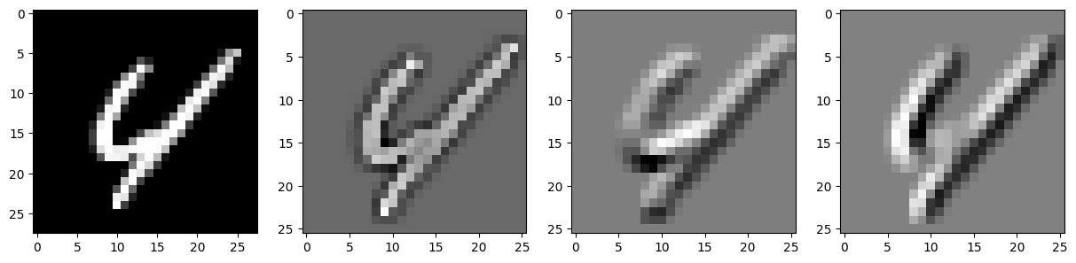
Edge Detector#
When the filter is applied to an image, it emphasizes the horizontal transitions from light to dark (or vice versa). When the filter slides over a horizontal edge in the image, the difference between the light and dark areas is emphasized by the positive and negative values in the filter, resulting in a high output value. In areas of the image without horizontal edges, the output values are close to zero. The second does the same but for a vertical edge.
[[ 1.  1.  1.]
 [ 0.  0.  0.]
 [-1. -1. -1.]]

[[ 1.  0. -1.]
 [ 1.  0. -1.]
 [ 1.  0. -1.]]
Architecture#
First, we start with layers, which you are already familiar with
The fully connected layer. It connects every neuron in the current layer to every neuron in the subsequent layer.
The softmax layer. It assigns probabilities to each class (numbers from zero to nine), indicating the likelihood of the input belonging to each class. The class with the highest probability is then predicted as the output class.
class FCLayer:
    def __init__(self, input_size, output_size):
        self.weights = np.random.randn(input_size, output_size) / np.sqrt(input_size)
        self.weights_update = np.zeros(self.weights.shape)

    def forward(self, input):
        self.input = input.copy()
        return np.dot(self.input, self.weights)

    def backward(self, grad):
        self.weights_update += np.outer(self.input, grad)
        return np.dot(grad, self.weights.T)

class Softmax:
    def forward(self, input):
        self.result = np.exp(input)/np.sum(np.exp(input))
        return self.result

    def backward(self, targets):
        return self.result - targets
In the next step, we introduce two new layers:
The convolution layer This layer creates num_filters different convolution masks/filters. Each filter is slid over the input image, multiplying the filter values with the corresponding pixel values in the image, and summing up the results. This process is repeated for every position of the filter on the image, resulting in a new output feature map.
The main advantage of convolutional layers is their ability to capture local patterns and spatial relationships within the input data. Unlike fully connected layers, which consider all input features equally, convolutional layers exploit the spatial structure of the data by sharing weights across different regions. This property makes convolutional layers particularly effective in tasks such as image classification, object detection, and image segmentation.
The maximum pooling layer A pooling window slides over the input feature map. At each position, the maximum value within the window is selected and becomes the output value for that region. The pooling window then moves to the next position, until the entire input is covered. The main purpose of maximum pooling is to downsample the input, reducing its spatial dimensions. This helps in reducing the computational complexity of subsequent layers and extracting the most salient features. By selecting the maximum value within each pooling window, maximum pooling retains the strongest feature activations, enhancing the robustness of the network to small spatial translations or distortions in the input.
In summary, convolutional and maximum pooling layers are essential building blocks of CNNs that enable the network to learn hierarchical representations of input data. By leveraging local patterns and spatial relationships, these layers extract meaningful features and contribute to the overall performance of the network in various computer vision tasks.
class ConvLayer:
    def __init__(self, num_filters, filter_size):
        self.num_filters = num_filters
        self.filter_size = filter_size
        self.filters = np.random.randn(num_filters, filter_size, filter_size) / (filter_size * filter_size)
        self.filters_update = np.zeros(self.filters.shape)

    def forward(self, input):
        self.input = input.copy()
        height, width = self.input.shape
        output_height = height - self.filter_size + 1
        output_width = width - self.filter_size + 1
        self.output = np.zeros((self.num_filters, output_height, output_width))

        for filter_idx in range(self.num_filters):
            for i in range(output_height):
                for j in range(output_width):
                    # The window is a local image region
                    window = self.input[i:i+self.filter_size, j:j+self.filter_size]
                    self.output[filter_idx, i, j] = np.sum(self.filters[filter_idx] * window)
        return self.output

    def backward(self, grad):
        _, output_height, output_width = grad.shape
        input_grad = np.zeros(self.input.shape)
        filter_grad = np.zeros(self.filters.shape)

        for filter_idx in range(self.num_filters):
            for i in range(output_height):
                for j in range(output_width):
                    window = self.input[i:i+self.filter_size, j:j+self.filter_size]
                    input_grad[i:i+self.filter_size, j:j+self.filter_size] += grad[filter_idx, i, j] * self.filters[filter_idx]
                    filter_grad[filter_idx] += grad[filter_idx, i, j] * window
        self.filters_update += filter_grad
        return input_grad

class MaxPoolLayer:
    def __init__(self, pool_size):
        self.pool_size = pool_size

    def forward(self, input):
        self.input = input.copy()
        num_channels, height, width = self.input.shape
        output_height = height // self.pool_size
        output_width = width // self.pool_size
        output = np.zeros((num_channels, output_height, output_width))

        for filter_idx in range(num_channels):
            for i in range(output_height):
                for j in range(output_width):
                    # The window is a local image region
                    window = self.input[filter_idx, i*self.pool_size:(i+1)*self.pool_size, j*self.pool_size:(j+1)*self.pool_size]
                    output[filter_idx, i, j] = np.max(window)
        return output

    def backward(self, grad):
        num_filters, height, width = self.input.shape
        output_height = height // self.pool_size
        output_width = width // self.pool_size
        input_grad = np.zeros(self.input.shape)

        for filter_idx in range(num_filters):
            for i in range(output_height):
                for j in range(output_width):
                    window = self.input[filter_idx, i*self.pool_size:(i+1)*self.pool_size, j*self.pool_size:(j+1)*self.pool_size]
                    max_val = np.max(window)
                    input_grad[filter_idx, i*self.pool_size:(i+1)*self.pool_size, j*self.pool_size:(j+1)*self.pool_size] = (window == max_val) * grad[filter_idx, i, j]
        return input_grad


class CNN:
    def __init__(self):
        self.conv_layer = ConvLayer(num_filters=6, filter_size=3)
        self.pool_layer = MaxPoolLayer(pool_size=2)
        # We get 13, because 28 - 3 + 1 = 26, and 26 / 2 = 13
        self.fc_layer = FCLayer(input_size=6*13*13, output_size=10)
        self.softmax = Softmax()

    def forward(self, x):
        x = self.conv_layer.forward(x)
        self.pool_output = self.pool_layer.forward(x)
        x = self.pool_output.flatten()
        x = self.fc_layer.forward(x)
        return self.softmax.forward(x)

    def backward(self, targets):
        grad = self.softmax.backward(targets)
        grad = self.fc_layer.backward(grad)
        # The fully connected layer had received a flatten input, so we have to reshape it back to the pooled shape
        grad = grad.reshape(self.pool_output.shape)
        grad = self.pool_layer.backward(grad)
        grad = self.conv_layer.backward(grad)
        return grad

    def update_weights(self, lr, batch_size):
        self.fc_layer.weights -= lr * self.fc_layer.weights_update / batch_size
        self.conv_layer.filters -= lr * self.conv_layer.filters_update / batch_size
        self.conv_layer.filters_update = np.zeros(self.conv_layer.filters.shape)
        self.fc_layer.weights_update = np.zeros(self.fc_layer.weights.shape)

cnn_model = CNN()
Train and Test#
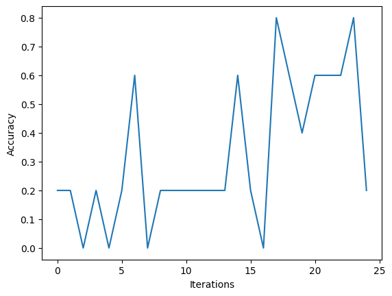
To keep the training and testing time small for demonstration purpose, we are only using a few iterations. For a real training, we would consider the whole dataset instead of just a randomly sampled subset. By further training we could significantly increase the accuracy. But this is not point of this notebook.
iterations = 25
train_batch_size = 10
test_batch_size = 5
lr = 0.1
accuracies = []

for i in range(iterations):
    # train
    random_samples = np.random.choice(len(X_train), train_batch_size)
    for idx in random_samples:
        cnn_model.forward(X_train[idx])
        cnn_model.backward(np.eye(10)[int(y_train[idx])])
    cnn_model.update_weights(lr, train_batch_size)

    # test
    accuracy = 0
    random_samples = np.random.choice(len(X_test), test_batch_size)
    for idx in random_samples:
        accuracy += np.argmax(cnn_model.forward(X_test[idx])) == int(y_test[idx])
    accuracies.append(accuracy / test_batch_size)
plt.xlabel('Iterations')
plt.ylabel('Accuracy')
plt.plot(accuracies)
[<matplotlib.lines.Line2D at 0x7f9ee1d86f90>]
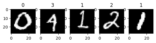
samples = np.random.choice(len(X_test), 5)
_, axs = plt.subplots(1,len(samples))
for i, sample in enumerate(samples):
    x = X_test[sample]
    axs[i].imshow(x, cmap='gray')
    axs[i].set_title(np.argmax(cnn_model.forward(x)))
Further Analysis#
We have seen the accuracy increase. That is good! Now, let us try to see, if we can gain a little bit of insight in what into a CNN.
First, we just visualize all the filter (convolution masks), our neural network has learned.
num_filters = cnn_model.conv_layer.num_filters
filter = lambda i : cnn_model.conv_layer.filters[i]

_, axs = plt.subplots(1, num_filters, figsize=(15, 10))
for i in range(num_filters):
    axs[i].imshow(filter(i), cmap='gray')
plt.show()
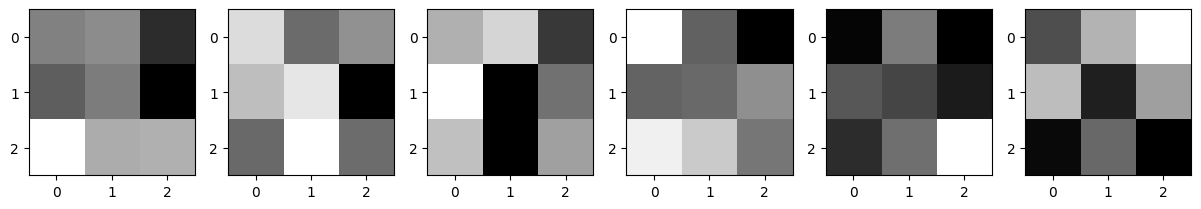
Depending on the outcome of your training, they might look random. Further training should improve that. Anyway, sometimes you can get already some idea of what features the filters might have learned. If not, we can just try to visualize them on our dataset.
Depending on the filter, we might find edge detectors, corner detectors, sharpening filters, etc.
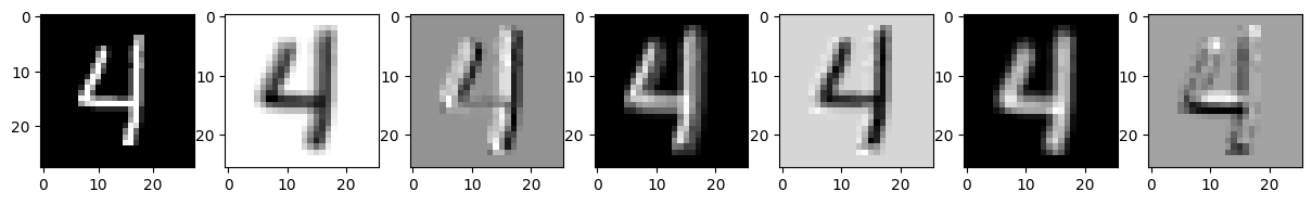
def gain_insight(sample):
    img = sample.reshape(28, 28)
    convolve = lambda i : convolve2d(img, filter(i), mode='valid')

    _, axs = plt.subplots(1, num_filters + 1, figsize=(15, 10))
    axs[0].imshow(img, cmap='gray')
    for i in range(num_filters):
        axs[i+1].imshow(convolve(i), cmap='gray')
gain_insight(X_train[7])
gain_insight(X_train[12])
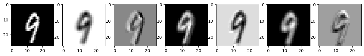
Have fun looking for features!