Clustering

Clustering is a fundamental technique in unsupervised machine learning that aims to group similar data points together based on their characteristics. One popular clustering algorithm is k-means, which partitions data into k distinct clusters.

The k-means algorithm starts by randomly initializing k cluster centroids. It then iteratively assigns each data point to the nearest centroid and updates the centroids based on the mean of the assigned points. This process continues until convergence, where the centroids no longer change significantly or a maximum number of iterations is reached.

K-means clustering is widely used in various domains, such as customer segmentation, image compression, anomaly detection, and recommendation systems. It provides a simple and efficient way to discover patterns and structure within datasets.

import numpy as np
from sklearn.datasets import make_blobs, make_moons
from sklearn.model_selection import train_test_split
import matplotlib.pyplot as plt

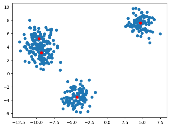
The first step, as always, is to get us some data. We are going to use the scikit library to generate us blobs of data. The red dots depict the cluster centers.

k = 4
X, y, centers = make_blobs(n_samples=500, centers=k, return_centers=True)
X_train, X_test, y_train, y_test = train_test_split(X, y, test_size=0.2)
plt.scatter(X_train[:, 0], X_train[:, 1])
plt.plot(centers[:, 0], centers[:, 1], 'ro')

[<matplotlib.lines.Line2D at 0x7fcdca506d50>]

Among all partitions \( C_0 \cup C_1 ... \cup C_k \), we find the one that minimizes:

\[ \min*{C_0 \cup C_1 ... \cup C_k} \sum*{i=1}^{k} \sum*{x \in C_i} ||x_i - \frac{1}{|C_i|} \sum*{x_j \in C_i} x_j ||^2 \]

• \( k \) are the number of clusters

• \( C_i \) is the i-th partition

• \( | C_i | \) is the number of samples belonging to \( C_i \)

• \( C_0 \cup C_1 ... \cup C_k \) is the union of all partitions

• \( x \in C_i \) means x in partition \( C_i \)

It calculates the sum of the squared distances between each data point and the mean of its assigned cluster. The goal is to minimize this sum by finding the optimal partitioning of the data into clusters. For the algorithm below, you can safely ignore this equation.

def kmeans(X, k, max_iter=100):
    # Choose k random samples as center of clusters
    centroids = X[np.random.choice(len(X), k, replace=False)]
    for i in range(max_iter):
        # Compute distance of each sample to each centroid
        dist = np.linalg.norm(X[:, None] - centroids, axis=2)
        # Assign each sample to the closest centroid
        labels = np.argmin(dist, axis=1)
        # Compute the new centroids by taking the mean of all samples assigned to each centroid
        new_centroids = np.array(
            [X[labels == i].mean(axis=0) for i in range(k)])
        if np.all(centroids == new_centroids):
            print(f'Converged after {i} iterations')
            break
        centroids = new_centroids
    return labels, centroids

labels, centroids = kmeans(X_train, k)
centroids = centroids[np.argsort(centroids[:, 0])]
plt.scatter(X_train[:, 0], X_train[:, 1], c=labels)
plt.plot(centers[:, 0], centers[:, 1], 'ro')
plt.plot(centroids[:, 0], centroids[:, 1], 'go')

Converged after 7 iterations

[<matplotlib.lines.Line2D at 0x7fcdc8260f90>]

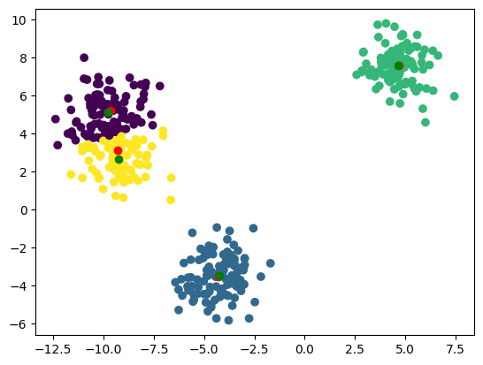
Now that we have our clusters (green dots), we can use them for classification.

def classify(X, centroids):
    dist = np.linalg.norm(X[:, None] - centroids, axis=2)
    return np.argmin(dist, axis=1)


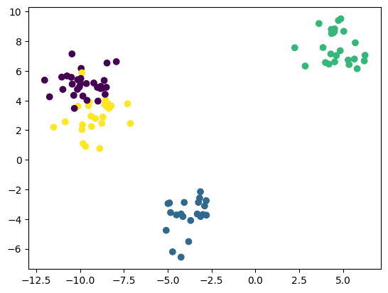
labels = classify(X_test, centroids)
plt.scatter(X_test[:, 0], X_test[:, 1], c=y_test)

<matplotlib.collections.PathCollection at 0x7fcdca539010>

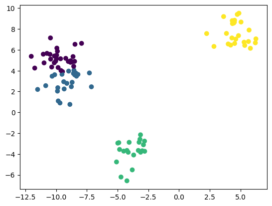
plt.scatter(X_test[:, 0], X_test[:, 1], c=labels)

<matplotlib.collections.PathCollection at 0x7fcdca38e390>

Disadvantages

1. You have to figure k out by yourself, although there are methods like the elbow method to help you with that.

2. We generated a blob dataset, because the shape of the data matters for k-means. If the data were not spherical, k-means would be a poor choice.

3. k-means cannot handle skewed data very well. By its nature, the centroids will always prefer bigger clusters.

Elbow Method

We iterate over multiple different values of \(k\) and look for the sweet spot, where the sum of distances between the samples and their cluster’s centroid starts to become low. The name becomes obvious if we look at the shape of the resulting graph.

inertia = []
for k in range(1, 10):
    labels, centroids = kmeans(X_train, k)
    inertia.append(np.linalg.norm(X_train - centroids[labels]))

plt.plot(range(1, 10), inertia)

Converged after 1 iterations
Converged after 7 iterations
Converged after 4 iterations
Converged after 7 iterations
Converged after 6 iterations
Converged after 4 iterations
Converged after 13 iterations
Converged after 8 iterations
Converged after 11 iterations

[<matplotlib.lines.Line2D at 0x7fcdca3566d0>]

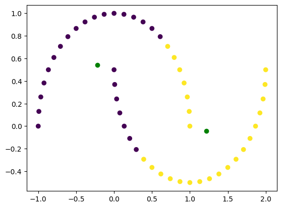
Non-spherical data

k = 2
X, y = make_moons(n_samples=50)
labels, centroids = kmeans(X, k)
plt.scatter(X[:, 0], X[:, 1], c=labels)
plt.plot(centroids[:, 0], centroids[:, 1], 'go')

Converged after 5 iterations

[<matplotlib.lines.Line2D at 0x7fcdc8158f50>]

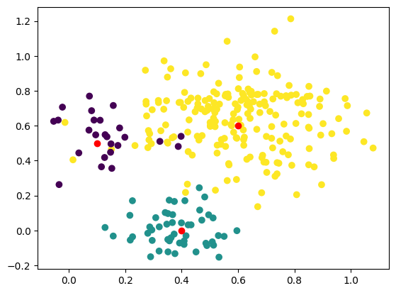
Skewed data

X, y, centers = make_blobs(n_samples=[25, 50, 200], cluster_std=[
                           0.1, 0.1, 0.2], centers=[(0.1, 0.5), (0.4, 0), (0.6, 0.6)], return_centers=True)
plt.scatter(X[:, 0], X[:, 1], c=y)
plt.plot(centers[:, 0], centers[:, 1], 'ro')

[<matplotlib.lines.Line2D at 0x7fcdc818e990>]

labels, centroids = kmeans(X, 3)
plt.scatter(X[:, 0], X[:, 1], c=labels)
plt.plot(centroids[:, 0], centroids[:, 1], 'go')

Converged after 9 iterations

[<matplotlib.lines.Line2D at 0x7fcdc8201fd0>]

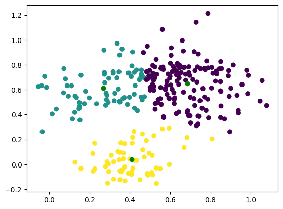
As you can see, k-means does not handle non-spherical data well and skewed data might also create a problem.

Nevertheless its simplicity and ease of use is often one of the first choices to cluster data. There are excellent libraries for this available.