P-NP Problems#
A decision problem is a computational problem that requires a yes-or-no answer. It involves determining whether a given input satisfies a specific property or condition. The goal is to determine whether a solution exists for a given instance of the problem. In the context of complexity theory, decision problems are often used to classify computational problems into different complexity classes, such as P (problems that can be solved in polynomial time) and NP (problems for which a solution can be verified in polynomial time).
In computer science, P (Polynomial Time) refers to the class of decision problems that can be solved by a deterministic Turing machine in polynomial time. This means that there exists an algorithm that can solve the problem in a time complexity that is polynomial in the size of the input.
On the other hand, NP (Nondeterministic Polynomial Time) refers to the class of decision problems for which a solution can be verified in polynomial time by a deterministic Turing machine. This means that given a potential solution, there exists an algorithm that can verify whether the solution is correct or not in a time complexity that is polynomial in the size of the input.
The relationship between P and NP is a fundamental question in computer science. The P vs NP problem asks whether every problem in NP can be solved in polynomial time. In other words, it asks whether P = NP. This problem remains unsolved, and it is considered one of the most important open questions in computer science.
import random
import numpy as np
import matplotlib.pyplot as plt
P (Polynomial) Example#
An example of a P problem is finding the maximum element in an array. This problem can be solved in polynomial time by iterating through the array once and keeping track of the maximum element encountered so far. The time complexity (how many steps are necessary to reach a solution) scales linearly with the size of the input.
# Given a set of integers, find the maximum element.
# It is easy to see, that it can be solved in linear time, meaning whatever the input is, it scales linearly.
integers = random.sample(range(1000), 1000)
def max_element(integers):
    max_el = integers[0]
    for i in range(1, len(integers)):
        if integers[i] > max_el:
            max_el = integers[i]
    return max_el

max_el = max_element(integers)

print("Integers:", integers[:10], "...")
print("Max element", max_el)
Integers: [541, 82, 138, 189, 609, 933, 927, 200, 348, 534] ...
Max element 999
NP (Nondeterministic Polynomial) Example#
The Subset Sum Problem: Given a set of integers and a target sum, the task is to determine whether there exists a subset of the integers that adds up to the target sum. While it is easy to verify a potential solution (a subset) by calculating its sum, finding the subset that adds up to the target sum requires checking all possible subsets, making it an NP problem.
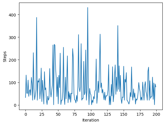
In the example below, you can see, that the average number of steps it takes to find a subset is 80 when the input length is 10. Of course, the implementation below is very naive and this is of course no proof, that it is a time-complex problem, but I dare you to find a deterministic algorithm which runs in polynomial time.
# Given a set of integers and a target sum, check if there exists a subset that sums to the target value.
def subset_sum(integers, target):
    global steps
    steps = 0
    def helper(index, current_sum):
        global steps
        steps += 1
        # Base case: if the current sum equals the target, return the subset
        if current_sum == target:
            return []
        # Base case: if the index is out of range or the current sum exceeds the target, return None
        if index >= len(integers) or current_sum > target:
            return None
        # Recursive case: try including the current integer in the subset
        subset = helper(index + 1, current_sum + integers[index])
        if subset is not None:
            subset.append(integers[index])
            return subset
        # Recursive case: try excluding the current integer from the subset
        return helper(index + 1, current_sum)
    return helper(0, 0), steps


hist = [subset_sum(random.sample(range(100), 10), random.randint(0, 100))[1] for _ in range(200)]
print('Average steps:', np.mean(hist))
plt.plot(hist)
plt.xlabel('Iteration')
plt.ylabel('Steps')
Average steps: 78.64
Text(0, 0.5, 'Steps')
Can you calculate/estimate, how many steps are needed in the worst case? Let us create such a worst case example and then do the math!
Our integers summed up are smaller than our target value. Thus the algorithm will go into every recursive branch.
subset, steps = subset_sum([1], 2)
print("Subset:", subset, "Steps:", steps)
subset, steps = subset_sum([1,2], 4)
print("Subset:", subset, "Steps:", steps)
subset, steps = subset_sum([1,2,3], 7)
print("Subset:", subset, "Steps:", steps)
subset, steps = subset_sum([1,2,3,4], 11)
print("Subset:", subset, "Steps:", steps)
subset, steps = subset_sum([1,2,3,4,5], 16)
print("Subset:", subset, "Steps:", steps)
Subset: None Steps: 3
Subset: None Steps: 7
Subset: None Steps: 15
Subset: None Steps: 31
Subset: None Steps: 63
In the worst case, the number of steps growth exponentially \( 2^{n+1} \), where \( n \) is the size of our input! While our approach is naive, the current best approach has a time complexity of \(2^{0.291n}\). It is a lot better, but still much. Let us plot it!
linear = np.linspace(0, 20, 20)
exp = 2**(0.291*linear)
plt.plot(linear, label='Linear')
plt.plot(exp, label='Exponential')
[<matplotlib.lines.Line2D at 0x7fc01eeb9bd0>]
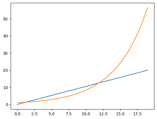
Even when the input is only of length 20, you can see the number of steps just exploding.
Remarks#
In the beginning I mentioned, that it is not proven that P = NP or that P != NP. The common assumption is indeed, that P != NP, because of what we have observed in reality.
If NP were proven to be equal to P, it would mean that efficient algorithms exist for solving NP problems, including prime factorization. This would render many encryption schemes vulnerable to attacks, potentially compromising the security of sensitive information, because many encryption algorithms rely on the difficulty of prime factorization. For example, the security of RSA encryption is based on the assumption that factoring large composite numbers into their prime factors is computationally infeasible.
Asymptotic Notation#
Asymptotic notation is a mathematical notation used in computer science and mathematics to describe the behavior of functions as their input size approaches infinity. It provides a concise way to analyze the efficiency and performance of algorithms.
There are several commonly used asymptotic notations, including Big O notation, Omega notation, and Theta notation. These notations allow us to classify algorithms based on their worst-case, best-case, or average-case time complexity. We only focus on Big O notation.
Big O notation (O): It represents the upper bound of the growth rate of a function. In other words, it describes the worst-case scenario of an algorithm’s time complexity. For example, if an algorithm has a time complexity of O(n), it means that the algorithm’s running time grows linearly with the input size.
Asymptotic notation allows us to compare the efficiency of different algorithms and make informed decisions when choosing the most suitable algorithm for a given problem. It helps us understand how the running time or space requirements of an algorithm scale with the input size, which is crucial for designing efficient and scalable software systems.
The mathematical formula for Big O notation is:
You have to read it like this: \( O(f) \) is the set of all functions \(g\), for which a positive constant \(c\) exists, such that they grow slower than \( c * f(n) \) after some \(n_0\).
Let’s look at an example on how we would categorize the function \(f(n) = 3n^3 + 2n^2 \):
\( f(n) = 3n^3 + 2n^2 \), \( c=5 \), \(n_0 = 1\), then for \( n \ge n_0 \)
\( n^2(1-n) \le 0 \rightarrow n^2 \le n^3 \rightarrow 2n^2 \le 2n^3 \rightarrow 3n^3 + 2n^2 \le 5n^3 \rightarrow 3n^3 + 2n^2 = O(n^3)\)
Examples from above#
max_elementalgorithm has a time complexity of \(O(n)\)subset_sumlet \(c=3\), then \(2^{n+1} = 2*2^n \le 3*2^n \rightarrow 2^{n+1} = O(n^2)\)