Formular Estimator#
The Formular Estimator is a powerful tool used in statistical analysis to estimate the relationship between variables. It is commonly used in regression analysis to determine the coefficients of a mathematical formula that best fits the data. In this Jupyter Notebook, we will explore the implementation of an easy example.
Let’s get started!
import numpy as np
import math
import matplotlib.pyplot as plt
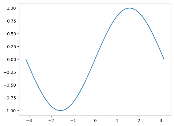
First, we start by creating our target function: a sine curve.
x = np.linspace(-math.pi, math.pi, 2000)
t = np.sin(x) # t for target
plt.plot(x,t)
[<matplotlib.lines.Line2D at 0x7fd319f46910>]
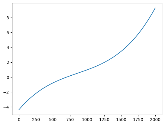
Let’s assume, we don’t know that this is a sine wave. We now roughly what we need, in this case we need a formula of third degree.
a = np.random.randn()
b = np.random.randn()
c = np.random.randn()
d = np.random.randn()

def sine(x):
    return a + b*x + c*x**2 + d*x**3
plt.plot(sine(x))
[<matplotlib.lines.Line2D at 0x7fd317b45810>]
Error Correction#
Right now, our plot doesn’t look like the sine wave we want. This is because all the weights in our network are set randomly at the start.
But don’t worry, we can fix this! We’re going to adjust these weights little by little to make our network’s output look more like a sine wave. This process is called “training”.
Think of it like tuning a guitar. When you first pick up a guitar, the strings might not be in tune. So, you pluck a string, listen to how it sounds, and then adjust the tuning peg a little bit. You keep doing this - pluck the string, listen, adjust - until the string sounds just right. That’s what we’re doing with our network: we’re “listening” to how far off its output is from a sine wave (this is the error), and then we’re “adjusting” the weights to make it sound better.
We’re lucky because we know what a sine wave looks like, so we know what we’re aiming for. We just need to keep adjusting our weights until we get there. This is the essence of training a neural network.
learning_rate = 1e-3
losses = []
for _ in range(2000):
    y = sine(x)
    loss = ((y - t)**2).mean()
    dLoss = 2.0 * (y - t)
    a -= learning_rate * dLoss.mean()
    b -= learning_rate * (dLoss * x).mean()
    c -= learning_rate * (dLoss * x ** 2).mean()
    d -= learning_rate * (dLoss * x ** 3).mean()

    losses.append(loss)
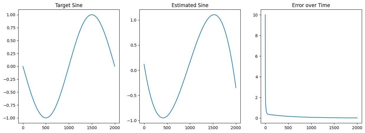
fig, axs = plt.subplots(1,3, figsize=(15, 5))
axs[0].set_title('Target Sine')
axs[0].plot(t)
axs[1].set_title('Estimated Sine')
axs[1].plot(sine(x))
axs[2].set_title('Error over Time')
axs[2].plot(losses)
print(f'Result: y = {a} + {b} x + {c} x^2 + {d} x^3')
Result: y = 0.16340132515792719 + 0.8800099553256612 x + -0.028189447599529478 x^2 + -0.09664021762921607 x^3