Reinforcement Learning#
Reinforcement learning is a subfield of machine learning that focuses on training agents to make sequential decisions in an environment to maximize a reward signal.
One of the challenges in reinforcement learning is defining the target value for optimization. Unlike classification tasks where we can use the correct label as a target, in reinforcement learning, a correct label is not readily available.
In this notebook, we will be using the gymnasium library, which provides a collection of environments for developing and testing reinforcement learning algorithms. Specifically, we will be working with the CartPole environment, where the goal is to balance a pole on a cart by applying appropriate actions.
import gymnasium as gym
import numpy as np
import matplotlib.pyplot as plt
import imageio
First of all, we are going to load the environment and investigate it.
env = gym.make('CartPole-v1', render_mode='rgb_array')
num_states = env.observation_space.shape[0]
num_actions = env.action_space.n
# The four states are: cart position, cart velocity, pole angle, pole angular velocity
# The two actions are: push cart to the left, push cart to the right
print('observation space:', num_states)
print('action space:', num_actions)
print('observation limit top', env.observation_space.high)
print('observation limit low', env.observation_space.low)
observation space: 4
action space: 2
observation limit top [4.8               inf 0.41887903        inf]
observation limit low [-4.8               -inf -0.41887903        -inf]
Random Search#
In our scenario, we have two possible actions: pushing the cart to the left or to the right.
0 signifies pushing the cart to the left
1 signifies pushing the cart to the right
Our strategy is straightforward. We take a random vector and multiply it with the observation state vector. If the result is greater than zero, we push the cart to the right. If it’s less than zero, we push it to the left. Each instance where the pole remains upright rewards us with a point, and we continue this process. The weight that results in the longest sequence of successful attempts is stored for future use.
def get_action(w, state):
    # return 0 or 1 based on the sign of the dot product between w and state
    return int(np.dot(w, state) >= 0)


weights = np.random.randn(num_states)
state, _ = env.reset()
action = get_action(weights, state)

print('weights:', weights)
print('state:', state)
print('action:', action)
weights: [-0.15629049 -0.50631288 -2.16371894  0.68413064]
state: [ 0.02211059 -0.03935274  0.03549513 -0.02043114]
action: 0
def run(env, w):
    state, _ = env.reset()
    rewards = 0
    for _ in range(1000):
        state, reward, done, _, _ = env.step(get_action(w, state))
        # every time the pole is upright, we get a reward of 1
        rewards += reward
        # done is True when the episode is over, either we reached the goal or the pole fell
        if done:
            break
    return rewards


def random_search(env, num_episodes):
    best_weights = None
    maximum_reward = 0
    rewards = []
    for _ in range(num_episodes):
        weights = np.random.randn(num_states)
        reward = run(env, weights)
        rewards.append(reward)
        # keep track of the best weights and the maximum reward
        if reward > maximum_reward:
            maximum_reward = reward
            best_weights = weights
    return best_weights, rewards
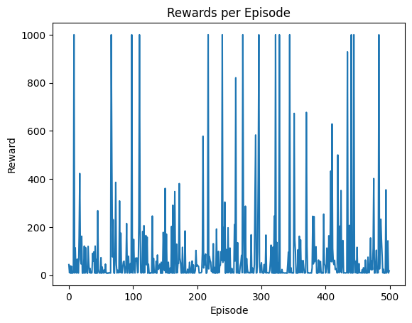
def plot_rewards(rewards):
    plt.plot(rewards)
    plt.xlabel('Episode')
    plt.ylabel('Reward')
    plt.title('Rewards per Episode')
    plt.show()
# In my experience, the sufficient weights are already gained after 50 episodes
best_weights, rewards = random_search(env, 500)
plot_rewards(rewards)
frames = []
for _ in range(5):
    state, _ = env.reset()
    done = False
    while not done:
        frame = env.render()
        frames.append(frame)
        state, _, done, _, _ = env.step(get_action(best_weights, state))
    imageio.mimsave('images/cartpole_random_search.gif', frames, fps=30)
Policy Learning#
The approach above is very simple and obviously does not scale to more complex problems. In a sense, we created a very limited neural network but instead of using gradient descent, we used a random optimization. Nevertheless, we can solve the problem smarter.
Policy Gradient methods are a type of Reinforcement Learning algorithms that directly optimize the policy (the strategy that the agent uses to determine the next action based on the current state). The key idea behind these methods is to push up the probabilities of actions that lead to higher rewards and push down the probabilities of actions that lead to lower rewards. Over time, this should lead to a policy that selects good actions more frequently.
First of all, we are going to build up our MLP again.
class FCLayer:
    def __init__(self, input_size, output_size, activation=None):
        self.relu = activation == 'relu'
        self.sigmoid = activation == 'sigmoid'
        self.tanh = activation == 'tanh'
        self.weights = np.random.randn(
            input_size, output_size) / np.sqrt(input_size)  # Xavier initialization
        self.bias = np.zeros(output_size)
        self.weight_update = np.zeros_like(
            self.weights)  # Gradients of the weight
        self.bias_update = np.zeros_like(self.bias)  # Gradients of the bias
        self.grad_counter = 0  # Number of gradients accumulated, used to average the gradients

    def forward(self, input):
        self.input = input.copy()
        self.y = np.dot(self.input, self.weights) + self.bias
        if self.relu:
            self.y[self.y < 0] = 0
        if self.sigmoid:
            self.y = 1.0 / (1.0 + np.exp(-self.y))
        if self.tanh:
            self.y = np.tanh(self.y)
        return self.y

    def backward(self, grad):
        if self.relu:
            grad[self.y <= 0] = 0
        if self.sigmoid:
            grad = grad * self.y * (1 - self.y)
        if self.tanh:
            grad = grad * (1 - self.y ** 2)
        self.weight_update += np.outer(self.input, grad)
        self.bias_update += grad
        self.grad_counter += 1
        return np.dot(grad, self.weights.T)

    def update_weights(self, learning_rate):
        self.weights -= learning_rate * self.weight_update / self.grad_counter
        self.bias -= learning_rate * self.bias_update / self.grad_counter
        self.grad_counter = 0  # Reset the gradient counter
        self.weight_update = np.zeros_like(self.weights)
        self.bias_update = np.zeros_like(self.bias)


class Network:
    def __init__(self, topology, learning_rate):
        self.learning_rate = learning_rate
        self.topology = topology

    def update_weights(self):
        for layer in self.topology:
            layer.update_weights(self.learning_rate)

    def forward(self, x):
        for layer in self.topology:
            x = layer.forward(x)
        return x

    def backward(self, x, y):
        for layer in self.topology:
            x = layer.forward(x)
        for layer in reversed(self.topology):
            y = layer.backward(y)
In this instance, the network architecture includes a genuine hidden layer. Previously, we only had an input layer and an output layer.
The final layer of our network has a single output that utilizes a sigmoid activation function. The sigmoid function is an excellent choice because it primarily outputs values close to 0 or 1.
topology = [
    FCLayer(4, 10, activation='relu'),
    FCLayer(10, 10),
    FCLayer(10, 1, activation='sigmoid')]
net = Network(topology=topology, learning_rate=0.5)
In reinforcement learning, an agent is an entity that interacts with an environment to learn and make decisions. The agent receives observations from the environment and takes actions based on those observations. The goal of the agent is to maximize a notion of cumulative reward over time.
To achieve this, the agent follows a policy, which is a mapping from states to actions. The policy guides the agent’s decision-making process by determining which action to take in a given state. The agent learns and improves its policy through a trial-and-error process, where it explores different actions and observes the resulting rewards.
Agents in reinforcement learning can be implemented using various algorithms, such as Q-learning, Deep Q-Networks (DQN), or policy gradients. Here, we will be looking at policy gradient learning.
class Agent():
    def __init__(self, net):
        self.net = net

    def act(self, state):
        # We interpret the output of the network as the probability of taking action 1 (going to the right)
        prob = self.net.forward(state)
        action = 1 if np.random.rand() < prob else 0
        return action, prob

    def _discount_rewards(self, rewards, gamma):
        discounted = np.zeros_like(rewards)
        reward = 0
        # We start from the end of the rewards list
        for t in reversed(range(len(rewards))):
            # We multiply the reward by gamma and add the reward at time t
            # This way, the reward at time t will have a weight of gamma^0, the reward at time t-1 will have a weight of gamma^1, and so on
            # Since gamma is less than 1, the rewards that are further in the past will have less weight
            reward = reward * gamma + rewards[t]
            discounted[t] = reward
        # By normalizing the rewards, we can make the training more stable
        discounted -= np.mean(discounted)
        discounted /= np.std(discounted)
        return discounted

    def train(self, episodes, gamma=0.99):
        total_rewards = []

        for _ in range(episodes):
            error_gradients = []
            episode_states = []
            episode_rewards = []
            done = False

            state, _ = env.reset()
            while not done:
                action, prob = self.act(state)
                # We want to encourage the actions that were taken
                # If the action was 1 (going to the right), we want the probability to be higher
                # If the action was 0 (going to the left), we want the probability to be lower
                # Action 1, Probability 1 -> Error: 0
                # Action 0, Probability 0 -> Error: 0
                # Action 1, Probability 0 -> Error: -1
                # Action 0, Probability 1 -> Error: 1
                error_gradients.append(prob-action)
                episode_states.append(state)
                state, reward, done, _, _ = env.step(action)
                episode_rewards.append(reward)

            # After every episode, we update the weights
            total_rewards.append(sum(episode_rewards))
            # We multiply the error gradients with the discounted rewards
            # This way, we encourage the actions that lead to a higher reward
            error_gradients = np.vstack(
                error_gradients) * self._discount_rewards(np.vstack(episode_rewards), gamma)

            for state, gradient in zip(episode_states, error_gradients):
                self.net.backward(state, gradient)
            # We update the weights in a batch
            # This helps to stabilize the training, since the weights are updated less frequently
            # and a single example does not have a big impact on the weights
            self.net.update_weights()

        return total_rewards
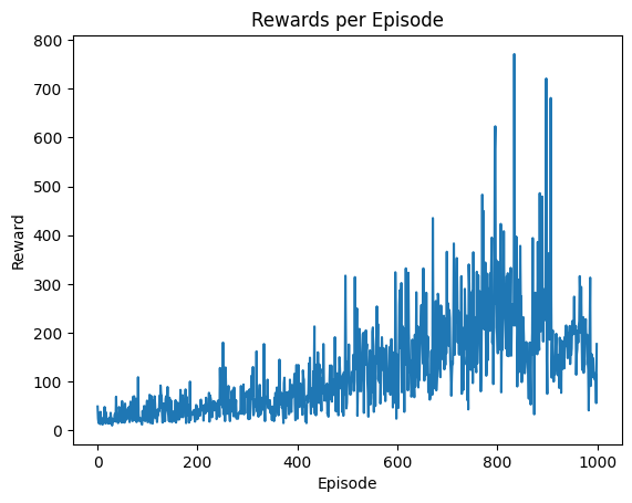
agent = Agent(net)
rewards = agent.train(1000)
plot_rewards(rewards)
frames = []
for _ in range(5):
    state, _ = env.reset()
    done = False
    while not done:
        frame = env.render()
        frames.append(frame)
        action, _ = agent.act(state)
        state, _, done, _, _ = env.step(action)
    imageio.mimsave('images/cartpole_policy_learning.gif', frames, fps=30)
While there are more sophisticated algorithms for tackling reinforcement learning challenges, such as Deep Q-Networks, they share a common principle with our approach - the notion of future rewards. Deep Q-Networks, for instance, employ a separate neural network to learn the policy. This network is trained to predict the maximum future reward for each possible action in a given state, and the action with the highest predicted reward is selected.
This concept of future rewards is fundamental to reinforcement learning. It’s based on the idea that actions taken now can have long-term consequences, and the goal is to choose actions that maximize the total reward over time, not just the immediate reward. This is what allows reinforcement learning agents to learn complex strategies that involve delayed gratification and planning ahead.