PyTorch

While it’s important to be familiar with specific frameworks, I believe it’s not beneficial to focus too much on any one in particular, as they often evolve or get replaced over time. We’ve seen this with Caffe, Theano, Tensorflow, Keras, and others. They all still exist, but currently, PyTorch is the most popular. If you’re interested in learning PyTorch, there are many comprehensive tutorials and guides available that are more detailed than this one.

In this guide, I aim to highlight the parallels between our custom-built MLP and an MLP implemented using PyTorch. We are going to inspect the same network architectures on the same data, that is why:

I strongly suggest going through the MLP notebook before proceeding with this one.

import numpy as np
import matplotlib.pyplot as plt
import torch
import torch.nn as nn

Binary Classification

def random_data():
    data = np.random.random_sample((100, 2))
    labels = (data[:, 0]-data[:, 1] < 0.3)

    d0 = data[labels == False]
    d1 = data[labels]

    targets = np.array([labels, 1-labels]).T
    return data, targets, labels, d0, d1


data, targets, labels, d0, d1 = random_data()
plt.plot(d0[:, 0], d0[:, 1], "bo")
plt.plot(d1[:, 0], d1[:, 1], "ro")

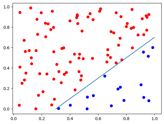
# Plot the decision boundary of a classifier: y = x - 0.3
x = np.linspace(0.3, 1, 2)
y = x - 0.3
plt.plot(x, y)

[<matplotlib.lines.Line2D at 0x7f3d1b22ff10>]

class MLP(nn.Module):
    def __init__(self, input_size, hidden_size, num_classes):
        super(MLP, self).__init__()
        self.fc1 = nn.Linear(input_size, hidden_size)
        self.fc2 = nn.Linear(hidden_size, num_classes)

    def forward(self, x):
        out = nn.functional.relu(self.fc1(x))
        out = nn.functional.sigmoid(self.fc2(out))
        return out


network = MLP(input_size=2, hidden_size=5, num_classes=2)
print("Network Structure:", network)

random_prediction = network(torch.tensor(data, dtype=torch.float32))
print("Random Prediction:", random_prediction.shape)

Network Structure: MLP(
  (fc1): Linear(in_features=2, out_features=5, bias=True)
  (fc2): Linear(in_features=5, out_features=2, bias=True)
)
Random Prediction: torch.Size([100, 2])

We’ve successfully created a Multilayer Perceptron (MLP) using PyTorch, and it’s structured similarly to the MLP we built from scratch. Let’s dissect what we’ve done:

1. We’ve created two fully connected layer objects. These are objects because they need to store certain information, such as gradients, which are essential for the learning process. This is similar to what we did in our custom-built MLP.

2. The activation functions ReLU and Sigmoid are used directly as function calls. They don’t need to store any state information, so they don’t need to be objects. They simply take the output of one layer and transform it to be the input for the next layer.

3. To get the output of our network for a given input, we simply call network(...) with the input. This runs the input through all the layers and activation functions of the network.

4. One of the advantages of using PyTorch is that we can feed all our data into the network at once. PyTorch, like most other deep learning frameworks, is designed to work with batches of data, allowing us to process multiple data points simultaneously. This can lead to significant speedups in training.

PyTorch provides a lot of functionality out of the box, like automatic differentiation and batch processing, which makes it easier and more efficient to work with, as you will see later.

def decision_boundary(f, d0, d1, diag=None):
    diag = diag or plt
    xx, yy = np.meshgrid(np.arange(0, 1, 0.01), np.arange(0, 1, 0.01))
    grid_data = np.c_[xx.ravel(), yy.ravel()]

    with torch.no_grad():
        zz = np.array([f(torch.tensor(p, dtype=torch.float32))
                      for p in grid_data]).reshape(xx.shape)
        diag.contourf(xx, yy, zz, alpha=0.3)
        diag.plot(d0[:, 0], d0[:, 1], "bo")
        diag.plot(d1[:, 0], d1[:, 1], "ro")


decision_boundary(lambda p: network(p)[0], d0, d1)

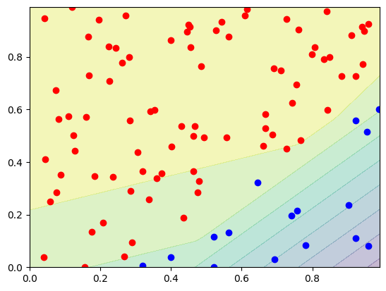
Remember, we do the same as in the MLP notebook, so we plan to create a classifier, which can separate two classes. We have used a simple gradient descent method, where we adapted our parameters using a learning rate. As Loss function we had used, the Mean Squared Error loss.

\[ MSE = \frac{1}{2}(y - y_t)^2 \]

optimizer = torch.optim.SGD(network.parameters(), lr=1)
criterion = nn.MSELoss()

# We convert the data to PyTorch tensors
input_tensor = torch.tensor(data, dtype=torch.float32)
target_tensor = torch.tensor(targets, dtype=torch.float32)

losses = []
for epoch in range(500):  # Epoch is the number of times we go through the entire dataset
    optimizer.zero_grad()  # weight_update = 0, bias_update = 0
    outputs = network(input_tensor)
    loss = criterion(outputs, target_tensor)
    losses.append(loss.item())
    loss.backward()  # Compute the gradients
    optimizer.step()  # Update the weights

fig, ax = plt.subplots(1, 2, figsize=(10, 5))
with torch.no_grad():
    correct = (network(input_tensor).argmax(dim=1) ==
               target_tensor.argmax(dim=1)).sum().item()
    print("Correct predicted: ", 1.0 * correct / len(data))
    decision_boundary(lambda p: network(p)[0], d0, d1, ax[0])

ax[1].set_title("Loss")
ax[1].plot(losses)

Correct predicted:  1.0

[<matplotlib.lines.Line2D at 0x7f3d0eb50c90>]

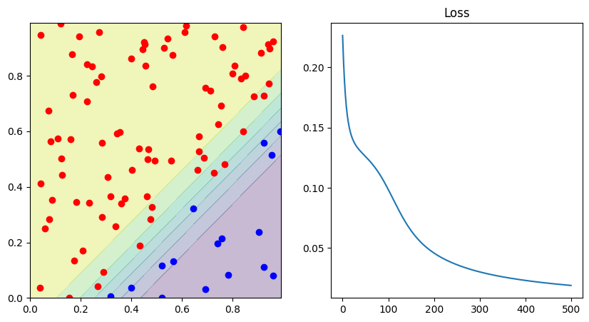
To validate the effectiveness of our PyTorch implementation, it’s beneficial to compare these graphs with those from the original notebook where we implemented the MLP from scratch.

The graphs should appear quite similar because the parameters we used for training the model in both cases are mostly identical. Specifically, we trained our model for 500 epochs in both notebooks using the same gradient descent approach.

Circle Data

def circular_random_data(radius=0.40):
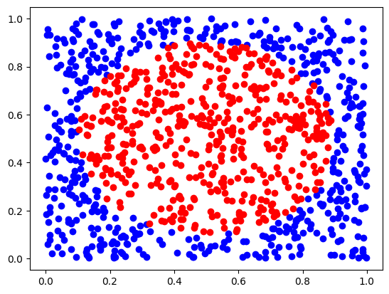
    data = np.random.random_sample((1000, 2))
    labels = (np.linalg.norm(data - 0.5, axis=1) < radius)

    d0 = data[labels == False]
    d1 = data[labels]

    # The value range of tanh is -1 to 1
    # -1 for negative class, 1 for positive class
    targets = 2*labels - 1
    return data, targets, labels, d0, d1


data, targets, labels, d0, d1 = circular_random_data()
plt.plot(d0[:, 0], d0[:, 1], "bo")
plt.plot(d1[:, 0], d1[:, 1], "ro")

[<matplotlib.lines.Line2D at 0x7f3d0eb6ae50>]

class CircularMLP(nn.Module):
    def __init__(self, input_size, hidden_size, num_classes, ):
        super(CircularMLP, self).__init__()
        self.fc1 = nn.Linear(input_size, hidden_size)
        self.fc2 = nn.Linear(hidden_size, num_classes)

    def forward(self, x):
        out = nn.functional.tanh(self.fc1(x))
        out = nn.functional.tanh(self.fc2(out))
        return out


network = CircularMLP(input_size=2, hidden_size=4, num_classes=1)
print("Network Structure:", network)

Network Structure: CircularMLP(
  (fc1): Linear(in_features=2, out_features=4, bias=True)
  (fc2): Linear(in_features=4, out_features=1, bias=True)
)

optimizer = torch.optim.SGD(network.parameters(), lr=0.05)
criterion = nn.MSELoss()

input_tensor = torch.tensor(data, dtype=torch.float32)
target_tensor = torch.tensor(targets, dtype=torch.float32).view(-1, 1)
print("Input Tensor Shape:", input_tensor.shape)
print("Target Tensor Shape:", target_tensor.shape)

Input Tensor Shape: torch.Size([1000, 2])
Target Tensor Shape: torch.Size([1000, 1])

losses = []
batch_size = 10
for epoch in range(500):
    loss_value = 0
    for i in range(0, len(data), batch_size):
        optimizer.zero_grad()
        outputs = network(input_tensor[i:i+batch_size])
        loss = criterion(outputs, target_tensor[i:i+batch_size])
        loss_value += loss.item() / len(data)
        loss.backward()
        optimizer.step()
    losses.append(loss_value)

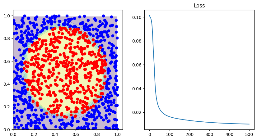
fig, ax = plt.subplots(1, 2, figsize=(10, 5))
with torch.no_grad():
    correct = np.sum([x == y for x, y in zip(np.sign(network(input_tensor)[:, 0]), target_tensor[:, 0])])
    print("Correct predicted: ", 1.0 * correct / len(data))
    decision_boundary(lambda p: network(p), d0, d1, ax[0])

ax[1].set_title("Loss")
ax[1].plot(losses)

/tmp/ipykernel_2465/1244354034.py:16: DeprecationWarning: __array_wrap__ must accept context and return_scalar arguments (positionally) in the future. (Deprecated NumPy 2.0)
  correct = np.sum([x == y for x, y in zip(np.sign(network(input_tensor)[:, 0]), target_tensor[:, 0])])

Correct predicted:  0.964

[<matplotlib.lines.Line2D at 0x7f3d0ea0bd10>]

In your everyday tasks, it’s rare that you’ll need to build a neural network from the ground up. There’s usually no necessity for this because there are many well-established libraries. These tools are designed to handle the complex mathematics and optimization processes involved in neural networks, which makes them less prone to errors compared to a custom-built solution.

However, having a fundamental understanding of the underlying concepts of neural networks is incredibly beneficial. This knowledge can be particularly useful when you’re debugging code. If something goes wrong while training a model or making predictions, understanding how the network operates can help you identify where the issue lies. For example, you might be able to recognize if the problem is due to incorrect data preprocessing, a poorly chosen activation function, or an issue with the way the network’s layers are connected.

In summary, while it’s not common to implement a neural network from scratch in your daily work, having a solid grasp of the principles behind neural networks can greatly assist in debugging and optimizing your models.