Multilayer Perceptron

import numpy as np
import matplotlib.pyplot as plt

Multilayer Perceptron is a type of artificial neural network that consists of multiple layers of interconnected nodes, called neurons. It is a feedforward neural network, meaning that the information flows in one direction, from the input layer to the output layer.

MLPs are widely used in various machine learning tasks, such as classification, regression, and pattern recognition. It is known for its ability to learn complex patterns and make accurate predictions.

The MLP uses a supervised learning technique called backpropagation for training. In backpropagation, the error is calculated between the predicted and actual output, and this error is propagated back through the network, starting from the output layer to the hidden layer(s), to adjust the weights for the next iteration.

Fully Connected Feed-Forward Network

The layers of an MLP typically include:

1. Input Layer: This is where the model receives its input features. Each node in this layer represents one feature.

2. Hidden Layer(s): These are layers between the input and output layers where the actual processing happens via a system of weighted ‘connections’. The most important aspect of the MLP is that these layers are “hidden”, meaning their values are not observable in the training set. Each node in these layers uses a nonlinear activation function, which allows the MLP to capture complex patterns.

3. Output Layer: This layer produces the final predictions of the model. The activation function used in this layer depends on the nature of the problem. For example, for a binary classification problem (our problem), a sigmoid function can be used.

Mathematics

In a neural network, each layer consists of multiple neurons, and each neuron is connected to all neurons from the previous layer. The input to a neuron is a weighted sum of the outputs of the neurons from the previous layer. If we consider all neurons in a layer, this operation can be represented as a matrix multiplication. The matrix contains the weights of the connections between the neurons in the current layer and the previous layer. The input data is multiplied by this weight matrix to give the initial output for each neuron in the current layer.

\[ y = f(X \times W) \]

Real-world data is often complex and non-linear. Activation functions introduce non-linearity into the network, allowing it to learn and model these complex patterns. Without an activation function, no matter how many layers the network has, it would still behave like a single-layer model because the composition of linear functions is still a linear function.

In our example, three types of activation functions are depicted:

1. Identity: This is a linear function where the output is the same as the input. It is used when we want to model a linear relationship. activation==None

2. ReLU: This function outputs the input directly if it’s positive; otherwise, it outputs zero. It’s widely used in deep learning models because it helps the model to train faster without sacrificing much accuracy.

3. Sigmoid: This function maps the input values into a range between 0 and 1, making it useful for outputting probabilities in binary classification problems.

We will look at them later separately!

class FCLayer:
    def __init__(self, input_size, output_size, activation=None):
        self.relu = activation == 'relu'
        self.sigmoid = activation == 'sigmoid'
        self.tanh = activation == 'tanh'
        self.weights = np.random.randn(
            input_size, output_size) / np.sqrt(input_size)  # Xavier initialization
        self.bias = np.zeros(output_size)
        self.weight_update = np.zeros_like(
            self.weights)  # Gradients of the weight
        self.bias_update = np.zeros_like(self.bias)  # Gradients of the bias
        self.grad_counter = 0  # Number of gradients accumulated, used to average the gradients

    def forward(self, input):
        self.input = input.copy()
        self.y = np.dot(self.input, self.weights) + self.bias
        if self.relu:
            self.y[self.y < 0] = 0
        if self.sigmoid:
            self.y = 1.0 / (1.0 + np.exp(-self.y))
        if self.tanh:
            self.y = np.tanh(self.y)
        return self.y

    def backward(self, grad):
        if self.relu:
            grad[self.y <= 0] = 0
        if self.sigmoid:
            grad = grad * self.y * (1 - self.y)
        if self.tanh:
            grad = grad * (1 - self.y ** 2)
        self.weight_update += np.outer(self.input, grad)
        self.bias_update += grad
        self.grad_counter += 1
        return np.dot(grad, self.weights.T)

    def update_weights(self, learning_rate):
        self.weights -= learning_rate * self.weight_update / self.grad_counter
        self.bias -= learning_rate * self.bias_update / self.grad_counter
        self.grad_counter = 0  # Reset the gradient counter
        self.weight_update = np.zeros_like(self.weights)
        self.bias_update = np.zeros_like(self.bias)


class Network:
    def __init__(self, topology, learning_rate):
        self.learning_rate = learning_rate
        self.topology = topology

    def update_weights(self):
        for layer in self.topology:
            layer.update_weights(self.learning_rate)

    def forward(self, x):
        for layer in self.topology:
            x = layer.forward(x)
        return x

    def backward(self, x, y):
        for layer in self.topology:
            x = layer.forward(x)
        for layer in reversed(self.topology):
            y = layer.backward(y)


network = Network(
    topology=[
        FCLayer(2, 5, activation='relu'),  # Input Layer
        FCLayer(5, 2, activation='sigmoid')  # Output Layer
    ],
    learning_rate=1)

Binary Classification

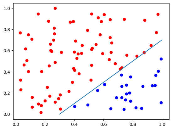
We generate randomly a synthetic dataset suitable for a binary classification problem. It consists of 100 2D samples. The optimal decision boundary is given by the equation:

\[ y = x - 0.3 \]

def random_data():
    data = np.random.random_sample((100, 2))
    labels = (data[:, 0]-data[:, 1] < 0.3)

    d0 = data[labels == False]
    d1 = data[labels]

    targets = np.array([labels, 1-labels]).T
    return data, targets, labels, d0, d1


data, targets, labels, d0, d1 = random_data()
plt.plot(d0[:, 0], d0[:, 1], "bo")
plt.plot(d1[:, 0], d1[:, 1], "ro")

# Plot the decision boundary of a classifier: y = x - 0.3
x = np.linspace(0.3, 1, 2)
y = x - 0.3
plt.plot(x, y)

[<matplotlib.lines.Line2D at 0x7fc91466c110>]

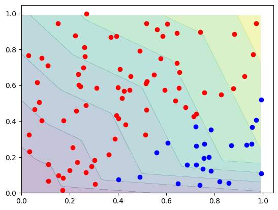
# Before training, the decision boundary is fuzzy and random
# You don't need to understand this function
def decision_boundary(f, d0, d1, diag=None):
    diag = diag or plt
    xx, yy = np.meshgrid(np.arange(0, 1, 0.01), np.arange(0, 1, 0.01))
    grid_data = np.c_[xx.ravel(), yy.ravel()]
    zz = np.array([f(p) for p in grid_data]).reshape(xx.shape)
    diag.contourf(xx, yy, zz, alpha=0.3)
    diag.plot(d0[:, 0], d0[:, 1], "bo")
    diag.plot(d1[:, 0], d1[:, 1], "ro")


decision_boundary(lambda p: network.forward(p)[0], d0, d1)

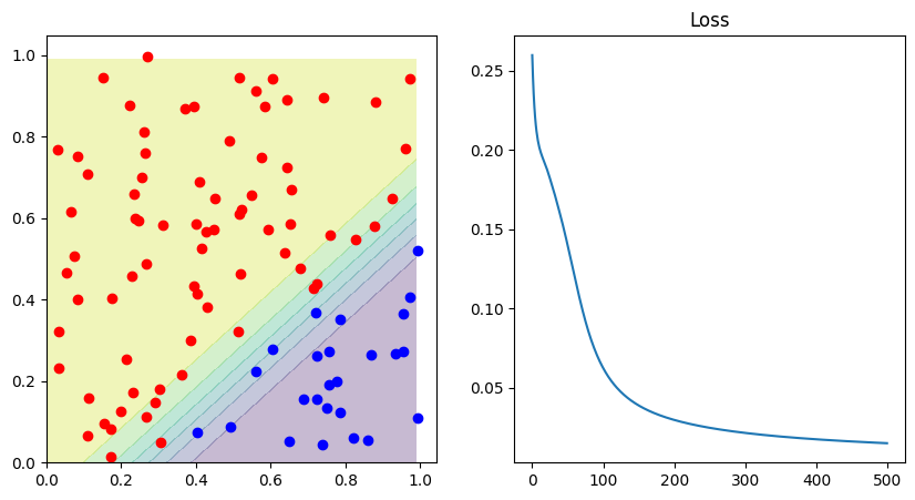
Training

The optimization of neural networks is called training and the algorithm is called backpropagation:

1. Forward Pass: The network makes a prediction based on the current weights. This prediction is compared to the actual output, and the difference is measured using a loss function. The goal is to minimize this loss.

2. Backward Pass (Backpropagation): In this step, the algorithm calculates how much each weight contributed to the loss, starting from the output layer and moving back towards the input layer. This is done by applying the chain rule of calculus to compute gradients (partial derivatives) of the loss function with respect to the weights and biases.

Once these gradients are known, the weights are updated in a way that reduces the loss. This is typically done using an optimization algorithm like gradient descent.

In simple terms, backpropagation is like a student learning from their mistakes. After answering a question (forward pass), the student checks their answer against the correct one. If the answer is wrong, the student reviews their solution to understand where they made a mistake (backward pass) and then corrects it. This process is repeated until the student is able to answer the question correctly.

In our example, we optimize the Mean Squared Error

\[ MSE = \frac{1}{2}(y - y_t)^2 \]

losses = []
for epoch in range(500):  # Epoch is the number of times we go through the entire dataset
    loss = 0
    for i in range(len(data)):
        out = network.forward(data[i])
        # Loss = 1/2(target - output)^2
        # We divide by 2 to make the derivative of the loss easier
        loss += 0.5 * np.sum((targets[i]-out)**2) / len(data)
        # dLoss/dOutput = -(target - output)
        network.backward(data[i], -(targets[i]-out))
    network.update_weights()
    losses.append(loss)

correct = np.sum([np.argmax(network.forward(x)) == np.argmax(y)
                 for x, y in zip(data, targets)])

print("Correct predicted: ", 1.0 * correct / len(data))
fig, ax = plt.subplots(1, 2, figsize=(10, 5))
decision_boundary(lambda p: network.forward(p)[0], d0, d1, ax[0])
ax[1].set_title("Loss")
ax[1].plot(losses)

Correct predicted:  0.99

[<matplotlib.lines.Line2D at 0x7fc9141a94d0>]

Toy around with the parameters. See how the network behaves, if you adapt the activation functions. Check what happens when you tweak the number of epochs.

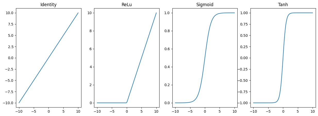
Activation Functions

def identity(x):
    return x


def relu(x):
    return np.maximum(0, x)


def sigmoid(x):
    return 1.0 / (1.0 + np.exp(-x))


x = np.linspace(-10, 10, 100)

_, axs = plt.subplots(1, 4, figsize=(15, 5))
axs[0].plot(x, identity(x))
axs[0].set_title('Identity')

axs[1].plot(x, relu(x))
axs[1].set_title('ReLu')

axs[2].plot(x, sigmoid(x))
axs[2].set_title('Sigmoid')

axs[3].plot(x, np.tanh(x))
axs[3].set_title('Tanh')

Text(0.5, 1.0, 'Tanh')

Circle Data

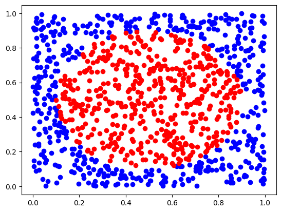
Next, we will look at non-linear data, especially, we will look at the first example of the Tensorflow Playground and try to recreate it.

Inspecting the parameters yields the following:

• 2 input neurons

• 4 hidden neurons

• 2 output neurons

• tanh activation function

• learning rate of 0.03

• batch size of 10

We will simplify the network a little bit and just use one output neuron, we have already seen how to neurons can be used, now let’s do the same just with one.

def circular_random_data(radius=0.40):
    data = np.random.random_sample((1000, 2))
    labels = (np.linalg.norm(data - 0.5, axis=1) < radius)

    d0 = data[labels == False]
    d1 = data[labels]

    # The value range of tanh is -1 to 1
    # -1 for negative class, 1 for positive class
    targets = 2*labels - 1
    return data, targets, labels, d0, d1


data, targets, labels, d0, d1 = circular_random_data()
plt.plot(d0[:, 0], d0[:, 1], "bo")
plt.plot(d1[:, 0], d1[:, 1], "ro")

[<matplotlib.lines.Line2D at 0x7fc90c95fe90>]

network = Network(
    topology=[
        FCLayer(2, 4, activation='tanh'),
        FCLayer(4, 1, activation='tanh')
    ],
    learning_rate=0.05)

losses = []
for epoch in range(500):
    loss = 0
    for i, (x, y) in enumerate(zip(data, targets)):
        out = network.forward(x)
        loss += 0.5 * (out-y)**2 / len(data)
        network.backward(x, out-y)
        if i % 10 == 0:
            network.update_weights()
    losses.append(loss)

correct = np.sum([np.sign(network.forward(x)) ==
                 y for x, y in zip(data, targets)])

print("Correct predicted: ", 1.0 * correct / len(data))
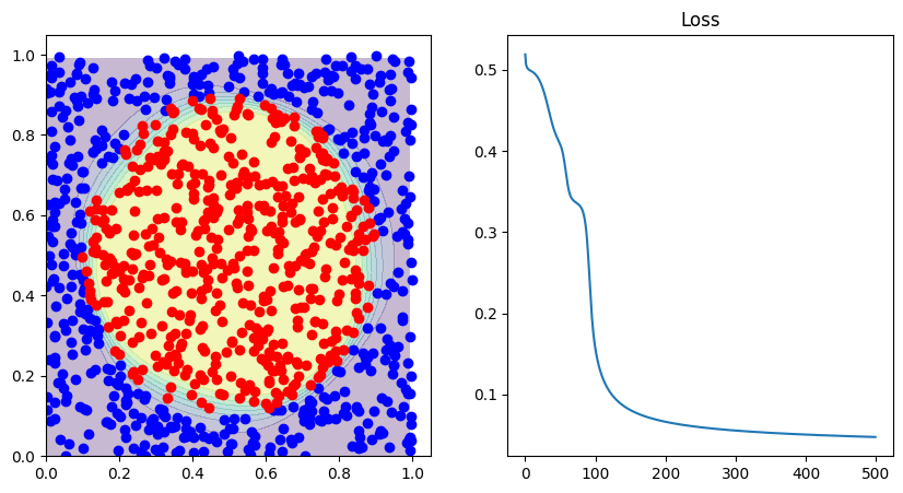
fig, ax = plt.subplots(1, 2, figsize=(10, 5))
decision_boundary(lambda p: network.forward(p), d0, d1, ax[0])
ax[1].set_title("Loss")
ax[1].plot(losses)

Correct predicted:  0.991

[<matplotlib.lines.Line2D at 0x7fc90cbf4e90>]

That’s it! By just slightly adapting our neural network, we could classify a completely different structure of data. We have seen how we can use two output neurons to classify two classes, but also how we can just use one. And we did not have to change the calculations whatsoever.