Principial Component Analysis#
Principial Component Analysis (PCA) is a statistical method to convert a set of observations of possibly correlated features into a set of values of linearly uncorrelated features called principal components. The number of principal components is less than or equal to the number of original features. The first principal component accounts for as much of the variability in the data as possible, and each succeeding component accounts for as much of the remaining variability as possible.
It is commonly used for dimensionality reduction by projecting each data point onto only the first few principal components to obtain lower-dimensional data while preserving as much of the data’s variation as possible. The first principal component can equivalently be defined as a direction that maximizes the variance of the projected data.
PCA identifies orthogonal axes (principal components) in the original feature space.
These axes are ordered by the amount of variance they explain.
By projecting the data onto these axes, we reduce the dimensionality while preserving the most important information.
To understand what we are doing and why we are doing it, we need a little excursion in the field of statistics
import numpy as np
import matplotlib.pyplot as plt
from pprint import pprint
from sklearn.datasets import load_iris
from sklearn.model_selection import train_test_split
from sklearn.linear_model import LogisticRegression
Expected Value, Variance and Covariance#
Features are the columns in our table, while data points are the rows
L=Sepal Length (cm) |
W=Sepal Width (cm) |
S=Petal Length (cm) |
T=Petal Width (cm) |
Species |
|---|---|---|---|---|
5.1 |
3.5 |
1.4 |
0.2 |
Setosa |
4.9 |
3.0 |
1.4 |
0.2 |
Setosa |
4.7 |
3.2 |
1.3 |
0.2 |
Setosa |
4.6 |
3.1 |
1.5 |
0.2 |
Setosa |
5.0 |
3.6 |
1.4 |
0.2 |
Setosa |
Expected value#
Let us calculate the expected values of all features
Variance#
It measures how far each number in the set is from the mean (average) and thus from every other number in the set. A high variance indicates that the feature is very spread out while a low variance indicates the opposite. We divide by \(n-1\) to not underestimate the variance.
The sepal width is more spread out than the sepal length and looking at the numbers, this becomes obvious.
Covariance#
The extension of the variance is the covariance. It is used to measure the linear relationship between two variables (data points). If the covariance is positive, it indicates that the two variables tend to increase or decrease together — that is, they’re directly proportional. If one variable tends to increase when the other decreases, the covariance is negative, indicating an inverse relationship. A covariance of zero suggests that the variables are independent of each other.
We have only looked at a subset of the iris flower dataset. So the values here must not necessarily represent the real dataset. But for this subset we can say the following:
The petal width (T) is independent of the other features.
The sepal length (L) and sepal width (W) are proportional to one other.
The other tend to behave inverse to one another.
# Lets validate our results
x = np.array([[5.1, 3.5, 1.4, 0.2], [4.9, 3.0, 1.4, 0.2], [
             4.7, 3.2, 1.3, 0.2], [4.6, 3.1, 1.5, 0.2], [5.0, 3.6, 1.4, 0.2]])
pprint(x)
print('mean:', np.mean(x, axis=0))
print('variance:', np.var(x, ddof=1, axis=0))
array([[5.1, 3.5, 1.4, 0.2],
       [4.9, 3. , 1.4, 0.2],
       [4.7, 3.2, 1.3, 0.2],
       [4.6, 3.1, 1.5, 0.2],
       [5. , 3.6, 1.4, 0.2]])
mean: [4.86 3.28 1.4  0.2 ]
variance: [0.043 0.067 0.005 0.   ]
Covariance Matrix#
pprint(np.cov(x, rowvar=False))
array([[ 0.043 ,  0.0365, -0.0025,  0.    ],
       [ 0.0365,  0.067 , -0.0025,  0.    ],
       [-0.0025, -0.0025,  0.005 ,  0.    ],
       [ 0.    ,  0.    ,  0.    ,  0.    ]])
The covariance matrix is a square (\( n\times n\)) matrix that provides a measure of the covariance between each pair of features in a dataset. In this matrix, each element \(C_{ij}\) represents the covariance between the feature \(x_i\) and \(x_j\). The diagonal elements of the covariance matrix (where i = j) are the variances of each feature.
On the diagonal, larger values in the covariance matrix indicate more variance.
On the non-diagonal, larger absolute values indicate a stronger linear relationship between two features.
def noise(x):
    return x + np.random.normal(0, 0.5, 100)


def plot(ax, y):
    ax.plot(x, y, 'o')
    ax.set_xlim(0, 10)
    ax.set_ylim(0, 25)


x = np.linspace(0, 10, 100)
ys = [noise(2*x), noise(-2*x+20), noise(10)]

fig, ax = plt.subplots(1, len(ys), figsize=(15, 5))
for i, y in enumerate(ys):
    plot(ax[i], y)
    pprint(np.cov(x, y))
    print('\n')
array([[ 8.58755909, 16.91255802],
       [16.91255802, 33.62306011]])


array([[  8.58755909, -17.35348144],
       [-17.35348144,  35.27430259]])


array([[ 8.58755909, -0.0410079 ],
       [-0.0410079 ,  0.33223664]])
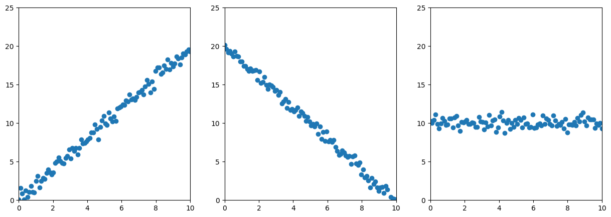
For simplicity, I omitted the decimal places.
We have variances along the x-axis (first element in all diagonals)
In the first two cases, we have variances along the y-axis (second element of the diagonal).
In the first example, x and y have a linear relation: If x increases, so does y.
In the second example, the relationship is inverted (negative values)
On the non-diagonal, larger absolute values indicate a stronger linear relationship between two features.
Geometrically, this means the non-diagonal values tell the “direction” of the data.
Eigenvalues and eigenvectors#
Let \(A\) be a \(n\times n\) matrix, then we call the scalar \(\lambda\) the eigenvalue and the non-zero vector \(v \in R^n\) the eigenvector for which \( Av = \lambda v \).
Multiplying the Matrix \(A\) with the eigenvector just scales the vector! The eigenvalue is just the scaling factor.
For the covariance matrix this means:
The eigenvector with the largest eigenvalue is the direction along which the data set has the maximum variance
Algorithm#
Finally, we can piece everything together:
PCA identifies orthogonal axes (principal components) in the original feature space.
These axes are ordered by the amount of variance they explain.
By projecting the data onto these axes, we reduce the dimensionality while preserving the most important information.
def pca(X):
    # Normalize the data
    X = (X - np.mean(X, axis=0))
    # Compute the covariance matrix
    cov = np.dot(X.T, X) / X.shape[0]
    # Perform singular value decomposition
    # U is the matrix of eigenvectors
    # S is the diagonal matrix of eigenvalues
    # V is the transpose of U
    U, S, V = np.linalg.svd(cov)
    return U, S, V


def project_data(X, U, k):
    # k is the number of dimensions to reduce to
    # U_reduced is the matrix of the first k eigenvectors
    U_reduced = U[:, :k]
    # Z is the projection of X onto the reduced dimension
    Z = np.dot(X, U_reduced)
    return Z
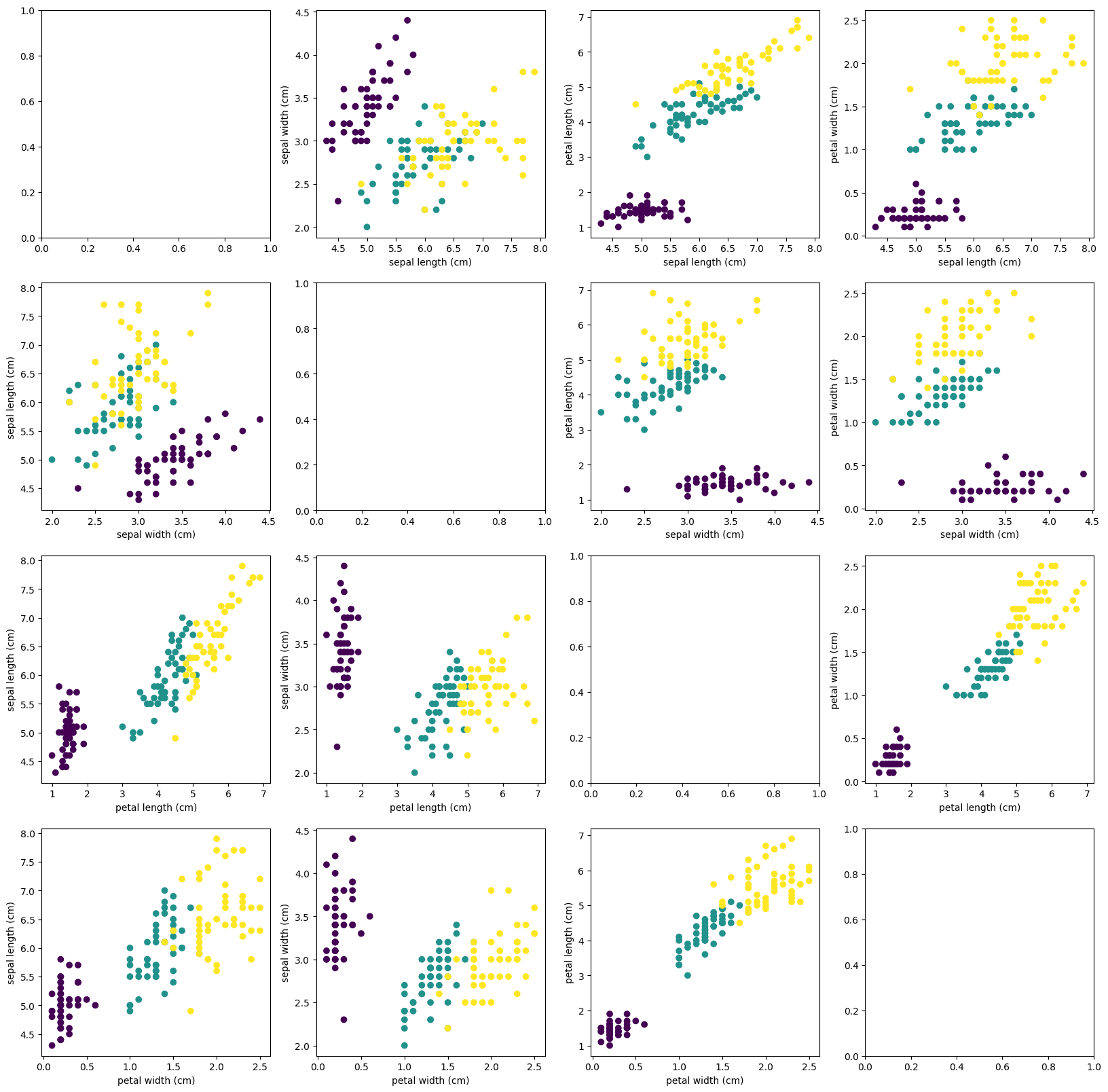
iris = load_iris()
print(iris.data.shape)

fig, axs = plt.subplots(4, 4, figsize=(20, 20))
for i in range(4):
    for j in range(4):
        if i != j:
            axs[i, j].scatter(iris.data[:, i], iris.data[:, j], c=iris.target)
            axs[i, j].set_xlabel(iris.feature_names[i])
            axs[i, j].set_ylabel(iris.feature_names[j])
(150, 4)
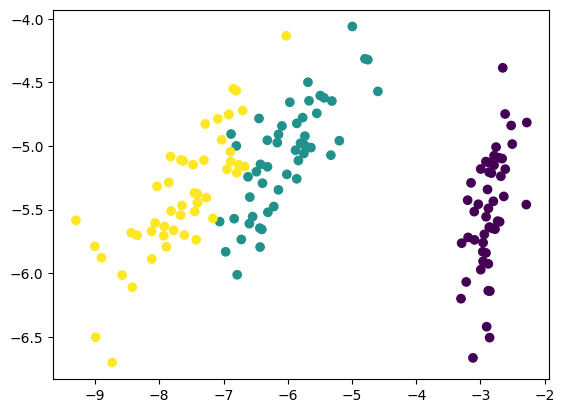
U, S, V = pca(iris.data)
# Project the four-dimensional data to two dimensions
Z = project_data(iris.data, U, 2)
print(Z.shape)
# We don't need to plot a grid, since we only have two dimensions left
plt.scatter(Z[:, 0], Z[:, 1], c=iris.target)
(150, 2)
<matplotlib.collections.PathCollection at 0x7f2ac1b66410>
# First, we are going to see how a logistic regression model performs on the data without dimensionality reduction
X_train, X_test, y_train, y_test = train_test_split(
    iris.data, iris.target, test_size=0.5)
clf = LogisticRegression()
clf.fit(X_train, y_train)
print(clf.score(X_test, y_test))
0.9466666666666667
# Next, we are going to see the performance with dimensionality reduction
X_train, X_test, y_train, y_test = train_test_split(
    Z, iris.target, test_size=0.5)
clf = LogisticRegression()
clf.fit(X_train, y_train)
print(clf.score(X_test, y_test))
0.96
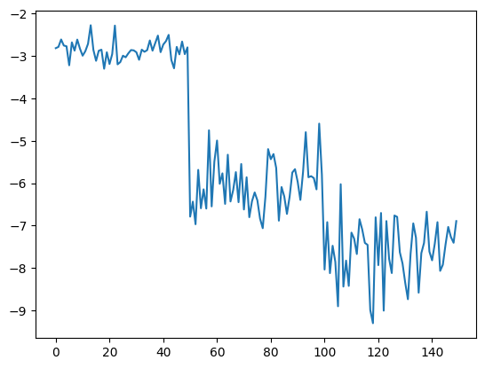
# Let us go to the extreme and project the data to one dimension
Z = project_data(iris.data, U, 1)
X_train, X_test, y_train, y_test = train_test_split(
    Z, iris.target, test_size=0.5)
clf = LogisticRegression()
clf.fit(X_train, y_train)
print(clf.score(X_test, y_test))
plt.plot(Z)
0.92
[<matplotlib.lines.Line2D at 0x7f2ac1ba6550>]
We’ve explored how PCA can effectively reduce the dimensionality of the iris flower dataset, preserving its fundamental characteristics. Although the iris flower dataset is a simple example, it demonstrates the significant role PCA can play in tasks like feature extraction or visualization. As with most tasks, it’s not necessary to build your own implementation from scratch. There are excellent libraries available that can perform PCA for you. However, understanding the underlying mathematics can provide valuable intuition about the process.