Softmax

In this chapter, we will look a little bit at the theory behind neural networks. The relation between the learning of networks and probability distributions.

import numpy as np
import matplotlib.pyplot as plt

Likelihood

Neural networks model probability distributions: \(P(y_i | \theta)\). This function calculates the probability to sample y given the parameters \(\theta\).

If you want to sample independent values from this distribution, e.g. calculate outputs using the network, we get \( P(y_0, y_1, ... | \theta) = \prod_i P(y_i|\theta)\).

In a neural network the \(\theta\) is represented by the weights. Improving the weights improves the model. This is called the Likelihood: \(L(y_0, y_1, .. | \theta) = P(y_0, y_1, .. | \theta)\).

Thus, the goal is to find the best parameters (weights) to achieve the best Likelihood:

\[\hat{\theta}^{MLE}=\underset{\theta}{\operatorname{argmax}} L(y_0, y_1, ..|\theta) \]

Combine the equations and you receive:

\[ \hat{\theta}^{MLE}=\underset{\theta}{\operatorname{argmax}} \prod_i L(y_i|\theta)\]

Since multiplications are difficult to use, we rewrite the function to use sums:

\[ \hat{\theta}^{MLE}=\underset{\theta}{\operatorname{argmax}} \sum_i \operatorname{\log} L(y_i|\theta)\]

Training a neural network means increasing the maximum log-likelihood!

Negative Log-Likelihood

If increasing the maximum log-likelihood is improving the network, so is decreasing the negative log-likelihood:

Usually, this is called the loss function. It is calculated, by summing the logarithms over the correct classes:

\[ NL(y_0, y_1, ..| \theta) = - \sum_i \operatorname{\log} L(y_i|\theta) \]

Example

Softmax:

\[ S(y_i) = \frac{e^y_i}{\sum_{j=1}^n e^y_i}\]

Let’s assume our network has three classes: Boat, Dog and cat.

The network has 3 output neurons and calculates for an input image the following:

\[y_0 = 5\]

\[y_1 = 2\]

\[y_2 = 1\]

If we apply softmax to the output of the network, we get:

\[ S(y_0) = 0.93623955 \]

\[ S(y_1) = 0.04661262 \]

\[ S(y_2) = 0.01714783 \]

where \(\sum S(y) = 1\)

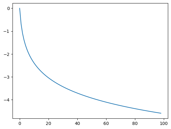
x = range(1,100)
plt.plot(-np.log(x))

[<matplotlib.lines.Line2D at 0x7f1d841a03d0>]

If in our example above our random sample is a boat, we get:

\[ NL(S(y_0)) = -log(0.93623955) = 0.06.. \]

If it would be a dog, we get:

\[ NL(S(y_1)) = -log(0.04661262) = 3.06.. \]

Wrong prediction have a high error. Thus if we minimize this function, we gradually improve our model.