Deep Q Learning#
This notebook was kindly provided by Nilau1998.
%%capture
# To keep the image size small, we only want the CPU version of PyTorch.
!pip install torch --index-url https://download.pytorch.org/whl/cpu
import collections
import random
import math
import matplotlib.pyplot as plt
import numpy as np
import gymnasium as gym
import torch.nn as nn
import torch

device = (
    "cuda" if torch.cuda.is_available() else
    "mps" if torch.backends.mps.is_available() else
    "cpu")
Bellman Equation#
Let us recap policy learning first. Policy learning attempts to learn functions which directly map an observation to an action:
Our agent had three methods, act, discount_rewards and train.
The agent runs a complete episode and stores all the rewards. After the episode is done, the rewards are weighted. Later rewards are weighted bigger than earlier rewards. The agent uses these rewards to calculate the gradient and optimize its network.
Unlike policy learning, Q-Learning attempts to learn the value of being in a given state, and taking a specific action there. In it’s simplest implementation, Q-Learning is a table of values for every state (row) and action (column) possible in the environment. We make updates to our Q-table using something called Bellman equation, which states that the expected long-term reward for a given action is equal to the immediate reward from the current action combined with the expected reward from the best future action taken at the following state.
\(Q(s, a)\) This represents the Q-value, which is the expected cumulative reward for taking action ‘a’ in state ‘s’. It is a function that maps a state-action pair to a value.
\(r\) This represents the immediate reward obtained when taking action ‘a’ in state ‘s’.
\(y\) This is the discount factor, which determines the importance of future rewards compared to immediate rewards. It is a value between 0 and 1.
\(\max Q(s', a')\): This represents the maximum Q-value for the next state ‘s’ and all possible actions ‘a’. It represents the estimated maximum future reward that can be obtained from the next state.
ReplayBuffer#
The ReplayBuffer is designed to store and manage experiences for training a reinforcement learning agent. It helps in stabilizing and improving the learning process. By randomly selecting a batch of experiences, it helps to break correlations between consecutive experiences.
class ReplayBuffer:
    def __init__(self, size):
        self.size = size
        self.memory = collections.deque([], maxlen=size)

    def sample(self, batch_size):
        return random.sample(self.memory, batch_size)

    def store_transition(self, transition):
        self.memory.append(transition)

    def __len__(self):
        return len(self.memory)
Epsilon Greedy-Policy#
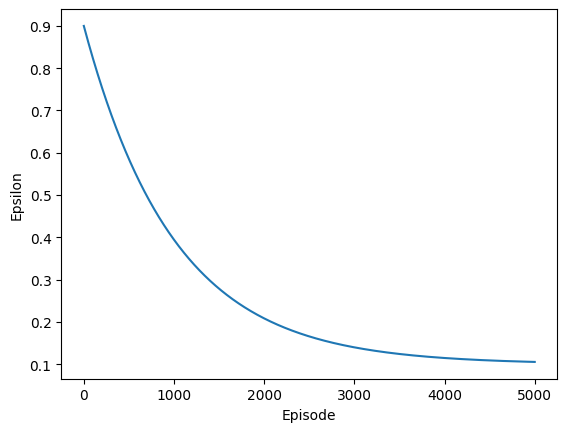
An epsilon-greedy policy is used to balance exploration and exploitation. Initially, the exploration rate (epsilon) is high to encourage exploration. It is gradually reduced over time, allowing the agent to exploit its learned policy more frequently. This annealing schedule helps transition from exploration to exploitation as training progresses.
def decay(epsilon_start, epsilon_end, epsilon_decay=1000):
    return lambda episode: epsilon_end + (epsilon_start - epsilon_end) * math.exp(-1. * episode / epsilon_decay)
eps_decay = decay(0.9, 0.1, 1000)

plt.plot([eps_decay(i) for i in range(5000)])
plt.xlabel("Episode")
plt.ylabel("Epsilon")
Text(0, 0.5, 'Epsilon')
Deep Q Network#
Architecture: The neural network consists of three fully connected layers. The first two layers use ReLU activation functions.
fc1: Input layer to the first hidden layer with 128 units.fc2: First hidden layer to the second hidden layer with 64 units.fc3: Second hidden layer to the output layer, with a number of units equal to the number of actions.
Optimizer: The Adam optimizer is used with a learning rate of 0.001.
class DeepQNetwork(nn.Module):
    def __init__(self, input_shape, n_actions, lr):
        super().__init__()
        self.fc1 = nn.Linear(*input_shape, 128)
        self.fc2 = nn.Linear(128, 64)
        self.fc3 = nn.Linear(64, n_actions)
        self.optimizer = torch.optim.Adam(self.parameters(), lr=lr)
        self.to(device)

    def forward(self, state):
        x = nn.functional.relu(self.fc1(state))
        x = nn.functional.relu(self.fc2(x))
        return self.fc3(x)

    @torch.no_grad()
    def predict(self, state):
        state = torch.tensor(state, dtype=torch.float32).to(device)
        return self.forward(state).argmax().item()
Agent#
The agent has two networks: dqn and target. The networks have the same architecture and and calculate the the \(Q(s,a)\). Basically, How good is action \(a\) in state \(s\). But they are used slightly different. dqn calculates the immediate Q-value while the target network is used to calculate \(\max Q(s',a')\).
act: Uses an epsilon-greedy policy to select actions. Epsilon is decayed over time to shift from exploration to exploitation. Initially it is more likely to choose a random action.
train : Updates the Q-network dqn using experiences sampled from the replay buffer. As loss function, we are using mean squared error between predicted and target Q-values. Periodically we soft update the target network parameters to stabilize training.
class Agent():
    def __init__(self, gamma, input_shape, n_actions, tau=0.05):
        self.gamma = gamma
        self.n_actions = n_actions
        self.memory = ReplayBuffer(10000)
        self.dqn = DeepQNetwork(input_shape, n_actions, 0.001)
        self.target = DeepQNetwork(input_shape, n_actions, 0.001)
        self.tau = tau

    def act(self, state, epsilon):
        if np.random.random() > epsilon:
            return self.dqn.predict(state)
        return np.random.choice(self.n_actions)

    def train(self, batch_size=64):
        if len(self.memory) < batch_size:
            return

        # sample random batch from memory
        batch = self.memory.sample(batch_size)
        states, actions, rewards, next_states, dones = zip(*batch)
        states = torch.tensor(np.array(states), dtype=torch.float32).to(device)
        actions = torch.tensor(actions, dtype=torch.int64).to(device)
        rewards = torch.tensor(rewards, dtype=torch.float32).to(device)
        next_states = torch.tensor(np.array(next_states), dtype=torch.float32).to(device)
        dones = torch.tensor(dones, dtype=torch.bool).to(device)

        # calculate the q values for the current state and the next state
        q_pred = self.dqn.forward(states).gather(1, actions.unsqueeze(-1)).squeeze(-1)
        q_next = self.target.forward(next_states).detach().max(dim=1).values
        # if the next state is terminal, the q value for the next state is 0
        q_next[dones] = 0.0
        q_target = rewards + (self.gamma * q_next)

        loss = nn.functional.mse_loss(q_target, q_pred).to(device)
        self.dqn.optimizer.zero_grad()
        loss.backward()
        self.dqn.optimizer.step()
        self.update_network_parameters()

    def update_network_parameters(self):
        # update the target network using the soft update
        target_value_state_dict = self.target.state_dict()
        value_state_dict = self.dqn.state_dict()
        for name in value_state_dict:
            target_value_state_dict[name] = value_state_dict[name] * \
                self.tau + target_value_state_dict[name]*(1-self.tau)
        self.target.load_state_dict(target_value_state_dict)
env = gym.make('CartPole-v1')
agent = Agent(gamma=0.99, input_shape=env.observation_space.shape, n_actions=env.action_space.n)
scores, epsilons, avg_scores = [], [], []
step = 0
for i in range(200):
score = 0
done, truncated = False, False
state = env.reset()[0]
while not done and not truncated:
action = agent.act(state, eps_decay(step))
next_state, reward, done, truncated, info = env.step(action)
score += reward
agent.memory.store_transition([state, action, reward, next_state, done])
agent.train(batch_size=64)
state = next_state
step += 1
scores.append(score)
avg_score = np.mean(scores[-100:])
avg_scores.append(avg_score)
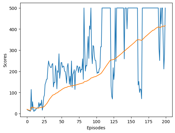
plt.plot(scores, label='Scores')
plt.plot(avg_scores, label='Average Scores')
plt.xlabel('Episodes')
plt.ylabel('Scores')
Text(0, 0.5, 'Scores')
Evaluation#
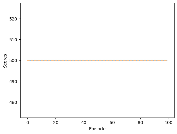
The model training stops when it consistently achieves the maximum score and the environment truncates. As expected, the average score continuously increases during training, indicating that the agent is effectively learning to control the CartPole. The epsilon value gradually decreases, meaning the agent relies more on its learned knowledge as training progresses.
During training, it was observed that the number of episodes significantly impacts performance and required fine-tuning. The model presented here needed 200 episodes, but using more episodes sometimes led to catastrophic forgetting, where the model’s performance deteriorated in later episodes. Automating this tuning process is challenging. One idea was to track the average score and stop training if it decreases, but this could prematurely halt training if the model is temporarily stuck in a local minimum and might improve in subsequent episodes.
n_eval_games = 100
eval_scores = []
for i in range(n_eval_games):
    score = 0
    done, truncated = False, False
    observation = env.reset()[0]
    while not done and not truncated:
        action = agent.act(observation, 0)
        observation_, reward, done, truncated, info = env.step(action)
        score += reward
        observation = observation_
    eval_scores.append(score)

plt.plot(eval_scores)
plt.plot([np.mean(eval_scores)] * n_eval_games, linestyle='--')
plt.xlabel('Episode')
plt.ylabel('Scores')
Text(0, 0.5, 'Scores')