Kalman Filter

The Kalman filter is a powerful mathematical tool used for estimating the state of a dynamic system from a series of noisy measurements. It is widely used in various fields such as robotics, navigation, finance, and control systems due to its ability to provide optimal estimates in real-time.

This notebook provides an in-depth exploration of the Kalman filter, including some theoretical foundations and a practical implementation. We will cover the following topics:

import numpy as np
from sklearn.model_selection import train_test_split
import matplotlib.pyplot as plt
import matplotlib.animation as animation
plt.rcParams["animation.html"] = "jshtml"

Gaussian Intuition

First, we need to talk about gaussian and the intuition behind them. A Gaussian distribution, also known as a normal distribution, is a way to describe how values are spread out. It is often used to represent real-world data that clusters around a central value.

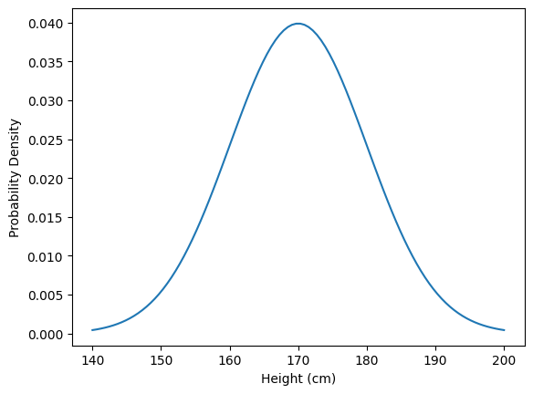
Imagine you are measuring the heights of a large group of people:

• Mean (\(\mu\)): The average height is 170 cm.

• Standard Deviation (\(\sigma\)): The standard deviation is 10 cm.

Given two gaussian distributions, the resulting Gaussian distribution after addition is:

\[ \mu = \mu_1 + \mu_2 \]

\[ \sigma = \sqrt{\sigma_1^2 + \sigma_2^2} \]

Given two gaussian distributions, the resulting Gaussian distribution after multiplication is:

\[ \mu = \frac{{\sigma_1^2 \mu_2 + \sigma_2^2 \mu_1}}{{\sigma_1^2 + \sigma_2^2}} \]

\[ \sigma = \frac{\sigma_1^2 \sigma_2^2}{\sigma_1^2 + \sigma_2^2} \]

class Gaussian:
    def __init__(self, mu, sigma):
        self.mu = mu
        self.sigma = sigma

    def plot(self):
        x = np.linspace(self.mu - 3*self.sigma, self.mu + 3*self.sigma, 100)
        y = np.exp(-0.5 * ((x - self.mu) / self.sigma)**2) / (self.sigma * np.sqrt(2*np.pi))
        return x,y

    def __add__(self, other):
        mu = self.mu + other.mu
        sigma = np.sqrt(self.sigma**2 + other.sigma**2)
        return Gaussian(mu, sigma)

    def __mul__(self, other):
        mu = (self.sigma**2 * other.mu + other.sigma**2 * self.mu) / (self.sigma**2 + other.sigma**2)
        sigma = np.sqrt(self.sigma**2*other.sigma**2 / (self.sigma**2 + other.sigma**2))
        return Gaussian(mu, sigma)

    def __repr__(self):
        return f'N(mu={self.mu}, sigma={self.sigma})'

measurement = Gaussian(170, 10)
plt.plot(*measurement.plot())
plt.xlabel('Height (cm)')
plt.ylabel('Probability Density')

Text(0, 0.5, 'Probability Density')

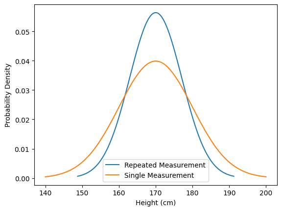
We repeat the measurement and obtain the same result. This should ideally increase our confidence that the average person’s height is indeed 170 cm. Mathematically, we can express this by combining our measurements, such as by multiplying the normal distributions. As a result, the uncertainty decreases (the variance is reduced).

repeated_measurement = measurement * measurement
plt.plot(*repeated_measurement.plot(), label='Repeated Measurement')
plt.plot(*measurement.plot(), label='Single Measurement')
plt.xlabel('Height (cm)')
plt.ylabel('Probability Density')
plt.legend()

<matplotlib.legend.Legend at 0x7fc6228268d0>

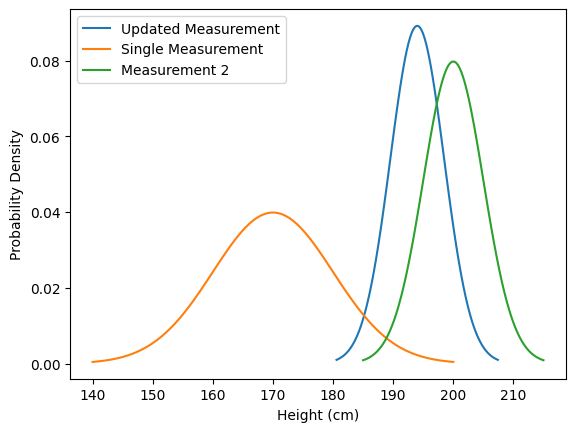
Suppose we take another measurement, and this time, the average height is 200 cm, which is higher than our initial measurement of 170 cm. We would then expect the true average height to lie somewhere between 170 cm and 200 cm. Consequently, the mean shifts towards the new measurement, and the uncertainty decreases.

measurement_2 = Gaussian(200, 5)
updated_measurement = measurement * measurement_2
plt.plot(*updated_measurement.plot(), label='Updated Measurement')
plt.plot(*measurement.plot(), label='Single Measurement')
plt.plot(*measurement_2.plot(), label='Measurement 2')
plt.xlabel('Height (cm)')
plt.ylabel('Probability Density')
plt.legend()

<matplotlib.legend.Legend at 0x7fc62247c810>

From Gaussian to Kalman Filter

The Kalman filter uses Gaussian distributions to represent the state and measurements.

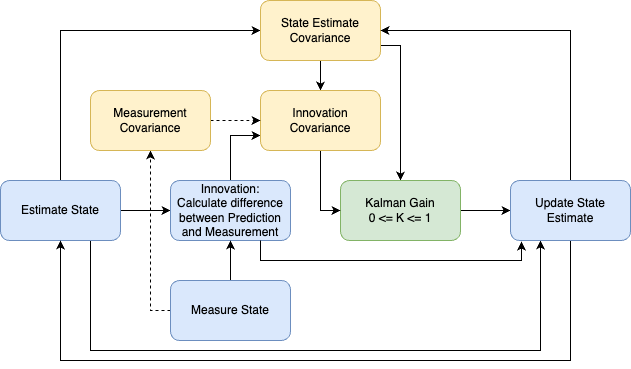
The flowchart visualizes the algorithm. I have categorized the boxes into three categories:

1. Main Steps (Blue): These boxes illustrate the primary steps involved in updating the state.

2. Covariances (Yellow): These boxes represent the measure of uncertainty.

3. Gain (Green): This central component is depicted in green.

Let’s consider a practical example where we estimate the position of a moving car. The car accelerates constantly, increasing its speed over time.

1. State Estimate: Initially, this can be random. We estimate the car’s position and velocity and calculate the uncertainty of this estimate using the covariance.

   • \(\mu_{\text{pred}} = A \mu_{\text{prev}}\)

   • \( \sigma_{\text{pred}}^2 = A \sigma_{\text{prev}}^2 A^T + Q \)

2. Measurement: We measure the car’s position and velocity, and optionally, the uncertainty of that measurement.

3. Innovation Calculation: We compute the innovation, which is the difference between the estimate and the measurement and the covariance of the innovation \(S\).

   • \( S = \sigma_{\text{pred}}^2 + \sigma_{\text{meas}}^2 \)

   • \( S^{-1} = \frac{1}{\sigma_{\text{pred}}^2 + \sigma_{\text{meas}}^2} \)

4. Kalman Gain: The gain indicates the reliability of the measurement versus the estimate. A high gain suggests low measurement uncertainty, and vice versa.

   • \(K = \frac{\sigma_{\text{pred}}^2}{\sigma_{\text{pred}}^2 + \sigma_{\text{meas}}^2}\), \( 0 \le K \le 1\)

5. Estimate Update: We update our initial estimate using the measurement, with the gain weighing the innovation.

   • \(\mu_{\text{update}} = \mu_{\text{pred}} + K (\mu_{\text{meas}} - \mu_{\text{pred}})\)

   • \(\sigma_{\text{update}}^2 = (1 - K) \sigma_{\text{pred}}^2\)

Car Tracking

This tracking example implements the flowchart from above in a 2-dimensional space. It is a more general version of the equations previously discussed. Could you implement the simplified version of this for a 1-dimensional case? How would it look?

Hints

• \(H\) would be just \(1\), since we would be dealing with scalars instead of matrices.

• The inverse of a matrix \(\mathbf{A} * \mathbf{A}^{-1} = \mathbf{I}\), where \(\mathbf{I}\) is the identity matrix. In the scalar world, this would be expressed as \(\mathbf{v} * \mathbf{v}^{-1} = 1 = \frac{\mathbf{v}}{\mathbf{v}} \)

• Remember the chapter about the PCA. The covariance is just the generalization of the variance. And the variance again is just a scalar.

dt = 1.0
steps = 15

# The state transition (A) matrix represents a constant velocity model, x_1 = x_0 + v_0 * dt
A = np.array([[1, dt],
              [0, 1]])

# Control input matrix (B) represents the change in velocity controlled by acceleration, u = 0.5 * a * t^2
B = np.array([[0.5 * dt**2], [dt]])

# state vector, [position; velocity]
x = np.array([[0], [0]])

# We directly measure the position, so the observation matrix (H) is just a selection matrix
H = np.array([[1, 0]])

# Process noise covariance (Q), represents the uncertainty in the model
Q = np.array([[0.25 * dt**4,    0.5 * dt**3],
              [0.5 * dt**3,     dt**2]])

# Initial state covariance
P = np.eye(2)

# Measurement noise covariance (R), represents the uncertainty in the measurements
R = np.array([[1]])

# Generate truth and noisy measurements
true_state = np.zeros((2, steps))
measurements = np.zeros(steps)
for t in range(1, steps):
    true_state[:, t] = np.dot(A, true_state[:, t-1]) + B.flatten()
    measurements[t] = true_state[0, t] + np.random.normal(0, 5)

estimates = np.zeros((2, steps))
gaussians = []

for t in range(steps):
    # Step 1, State estimate
    x = A @ x
    P = A @ P @ A.T + Q
    gaussians += [Gaussian(x[0, 0], np.sqrt(P[0, 0]))]

    # Step 2, Measurement
    z = np.array([[measurements[t]]])

    # Step 3, Innovation
    y = z - H @ x
    # S is the innovation covariance, the sum of the measurement covariance and the estimated covariance
    S = H @ P @ H.T + R

    # Step 4, Kalman Gain
    K = P @ H.T @ np.linalg.inv(S)
    # Step 5, Update the state estimate
    x = x + K @ y
    P = (np.eye(2) - K @ H) @ P
    estimates[:, t] = x.flatten()

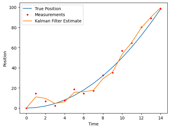
plt.plot(true_state[0], label='True Position')
plt.plot(measurements, 'r.', label='Measurements')
plt.plot(estimates[0], label='Kalman Filter Estimate')
plt.xlabel('Time')
plt.ylabel('Position')
plt.legend()

<matplotlib.legend.Legend at 0x7fc6224fb0d0>

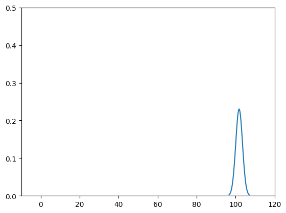
class Visualizer:
    def __init__(self, gaussians):
        self.gaussians = gaussians
        self.fig, self.ax = plt.subplots()
        self.ax.set_xlim(-10, 120)
        self.ax.set_ylim(0, 0.5)
        self.lines, = self.ax.plot(*gaussians[0].plot())

    def animate(self, t):
        g = self.gaussians[t]
        x, y = g.plot()
        self.lines.set_data(x, y)
        return self.lines,

    def plot(self):
        return animation.FuncAnimation(self.fig, self.animate, frames=len(self.gaussians), blit=True)

ev = Visualizer(gaussians)
ev.plot()

Once Loop Reflect