Convolution

This notebook explores various concepts related to image filtering and convolution. It demonstrates the use of linear filters, such as box filters and Gaussian filters, and explains their properties and applications.

By the end of this notebook, you will have a solid understanding of image filtering, convolution, and the different types of filters commonly used in image processing. You will also be familiar with efficient implementation techniques and the properties of convolution.

Let’s dive into the world of image filtering and convolution!

Impulse Response

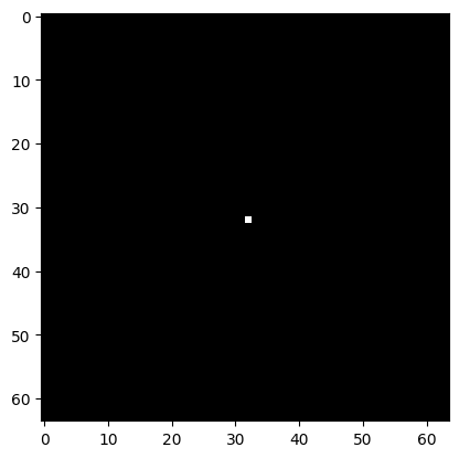
An impulse is just an image consisting of all zeros, except for a single pixel that has the value 1.0, at the center. Impulse responses fully characterize linear filters, as we shall see below.

import numpy as np
import matplotlib.pyplot as plt
import scipy.ndimage as img
from PIL import Image

def imrow(*args):
    _, axs = plt.subplots(1,len(args))
    for i, im in enumerate(args):
        axs[i].imshow(im, cmap='gray')

# 2D array representing an impulse
impulse = np.zeros((64,64))
impulse[32,32] = 1.0
plt.imshow(impulse,  cmap='gray')

<matplotlib.image.AxesImage at 0x7f345bf354d0>

Box Filter and Gaussian Filter

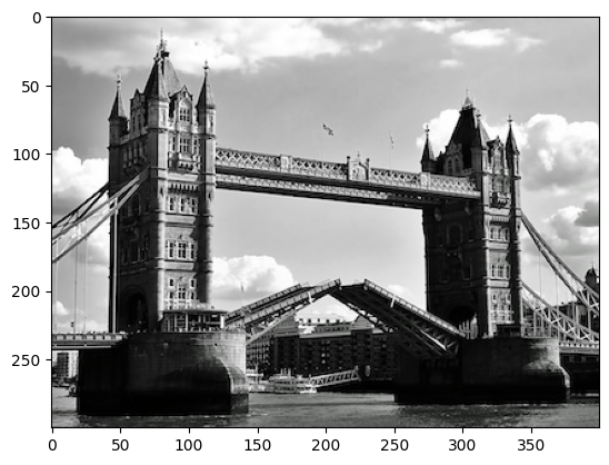
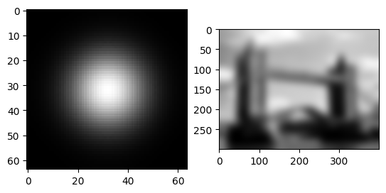
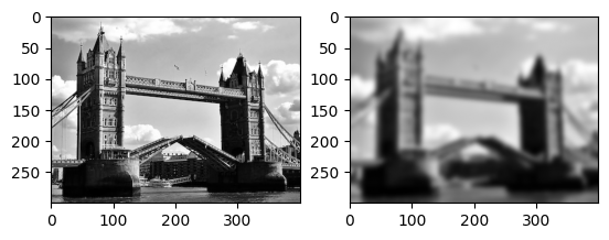
Let’s start by loading an image and inspecting it. We are looking at a grayscale image

image = np.array(Image.open('images/bridge.jpeg'))
print(image.shape, image[:1,:1,:], np.max(image))
plt.imshow(image)

(300, 400, 3) [[[175 175 175]]] 255

<matplotlib.image.AxesImage at 0x7f345be37e50>

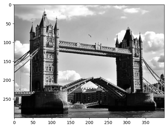
flatten = np.average(image, axis=2) / 255.0
print(flatten.shape, flatten[:1,:1], np.max(flatten))
plt.imshow(flatten, cmap='gray')

(300, 400) [[0.68627451]] 1.0

<matplotlib.image.AxesImage at 0x7f345bebb390>

Let’s start with a box filter (or uniform filter). You can think of this as “local averaging” of the pixels of an image. That is, you replace each pixel with an average of the pixels around it.

imrow(img.uniform_filter(impulse, 5.0), img.uniform_filter(flatten, 5.0))

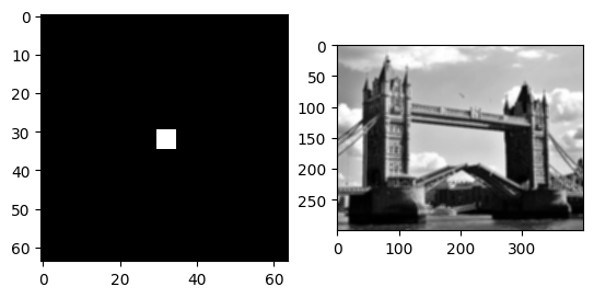
Can you spot what is happening? We are averaging over the image. The filter’s response can be seen very clearly on the impulse image.

In the next stepp, we use a different filter, than just a stupid box filter. We use a gaussian filter.

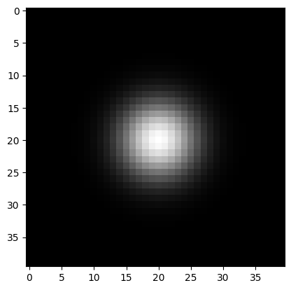
A Gaussian filter is similar to a box filter, but instead of taking an average over a neighborhood, you take a weighted average. The further a pixel is away from the center pixel, the less it contributes to the average. The weight of the averages is given by the Gaussian function (see below). Using it has numerous mathematical and practical advantages. This is one of the most common filters used in practice. You can “read off” the weights in the impulse response.

imrow(img.gaussian_filter(impulse, 10.0), img.gaussian_filter(flatten, 10.0))

The impulse response is important because it completely characterizes a linear shift invariant filter. Why? Because we can decompose an image into impulses, then apply the impulse response to each filter, and then add it all up again.

(definitions)

Let the input image be \(I\) and pixel \((i,j)\) given by \(I_{ij}\).

Write the impulse signal as \(\delta\).

Also, let \(S_{ij}\) be a filter that shifts the image such that the pixel at the origin ends up at position \(i,j\). It’s easy to see that \(S\) is also a linear filter.

Now,

\( I = \sum S_{ij}[I_{ij}\cdot\delta] \)

(impulse response and filters)

\( F[I] = F[\sum S_{ij}[I_{ij}\delta]] \)

By linearity:

\( = \sum F[S_{i,j} [I_{ij}\delta]] \)

By shift invariance:

\( = \sum S_{i,j}[ F[I_{ij}\delta] ] \)

By linearity, since \(I_{ij}\) is just a number:

\( = \sum S_{i,j} [I_{ij} F[\delta] ] \)

Here, \(F[\delta]\) is the impulse response.

(equivalence)

Therefore, applying a linear filter is equivalent to just summing up its impulse response.

(convolution)

The operation of combining an image with the impulse response of a filter is called the convolution.

Ignoring boundary conditions, for infinitely large 1D signals, it is written as:

\( (x * y)~_i = \sum_{j=-\infty}^{\infty} x_j y_{i-j} \)

(properties of convolutions)

Convolution has the following properties:

• commutativity: \(x * y = y * x\)

• associativity: \(x * (y * z) = (x * y) * z\)

• distributivity: \(x * (y + z) = x * y + x * z\)

• scalar multiplication: \(\alpha (x * y) = (\alpha x) * y = x * (\alpha y)\)

(2D convolution)

In 2D, convolution is defined analogously.

These properties carry over to linear shift invariant filters, since convolutions and linear shift invariant filters are equivalent.

(cross-correlation)

Note that there is a closely related operation where the minus sign has been replaced with a plus, the cross-correlation:

\( (x \star y)~_i = \sum_{j=-\infty}^{\infty} x_j y_{i+j} \)

The minus sign has the effect of “flipping” the mask around. This is also a useful operation, but the algebraic identities above don’t quite hold anymore.

(convolution in the library)

Convolution is implemented by the convolve function.

Let us check that applying linear filter \(g(\cdot,5)\) is the same as convolving with its impulse response.

That is, \(g(x,5) = x * g(\delta,5)\)

mask = img.gaussian_filter(impulse, 5.0)
convolved_image = img.convolve(flatten, mask)
filtered_image = img.gaussian_filter(flatten, 5.0)

imrow(convolved_image, filtered_image)
print(np.amax(abs(filtered_image-convolved_image)))

4.3298697960381105e-15

Composition of Filters

Let us check associativity of filters. This is a very useful property of linear filters because instead of applying a sequence of tilers, we can pre-compose the filters and then just apply the filter once.

# composition of linear filters
result1 = img.convolve(img.convolve(flatten,mask),mask)
result2 = img.convolve(flatten,img.convolve(mask,mask))
imrow(result1,result2)
print(np.amax(abs(result1-result2)))

2.9170629032293505e-06

(composition of Gaussian filters)

Does this work for Gaussian filters?

Yes, but there is one small thing to watch out for: the parameter that we give to the Gaussian filter does not quite combine in the way we expect. Applying two Gaussian filters of width 5 is equivalent to applying on one of width \(\sqrt{5^2+5^2}\).

(Looking at the definition of the Gaussian and Gaussian filter below, work out for yourself why these parameters behave like that.)

gf = img.gaussian_filter
result1 = gf(gf(flatten,5.0),5.0)
result2 = gf(flatten,np.sqrt(5**2+5**2))
imrow(result1,result2)
print(np.amax(abs(result1-result2)))

3.710844170035088e-05

Separability

Many filtes are separable. That is, instead of convolving with a 2D mask, we can convolve with two 1D masks.

For Gaussian filters, we can actually specify the width and the height of the filter separately. Applying two filters of shape (5,0) and (0,5) is equivalent to applying one filter of shape (5,5).

# horizontal and vertical Gaussians
vf = gf(impulse,(5.0,0.0))
hf = gf(impulse,(0.0,5.0))
imrow(impulse, vf,hf)

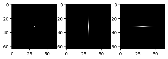
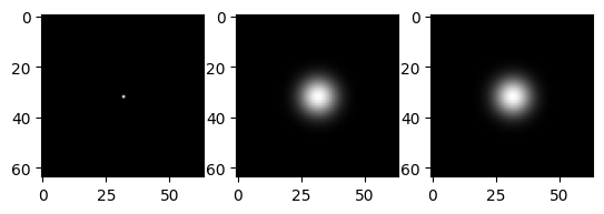
The convolution of these two filters is the same as a Gaussian.

# convolution of horizontal and vertical Gaussians
imrow(vf,hf,img.convolve(vf,hf))

These properties now carry over to the filters themselves.

Note that \( g(\cdot,(5,0)) \) is implemented more efficiently than \(g(\cdot,(5,5))\).

# separable convolution
imrow(impulse,gf(impulse,(5.0,5.0)),gf(gf(impulse,(5.0,0.0)),(0.0,5.0)))

# separable convolution
imrow(gf(flatten,(5.0,5.0)),gf(gf(flatten,(5.0,0.0)),(0.0,5.0)))

Gaussians

We keep talking about Gaussian filters, but haven’t really looked at what those weights are.

They are given by the following simple function.

xs = np.arange(-5.0,5.0,0.25)
ys = np.exp(-xs**2/2.0)
plt.plot(xs,ys)

[<matplotlib.lines.Line2D at 0x7f34588662d0>]

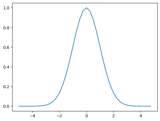
The general formula is:

\( G(x) = (2\pi\sigma^2)^{-1/2} e^\frac{-(x-\mu)^2}{2\sigma^2} \)

This generalizes to multiple dimensions by just using vectors for \(\mu\) and \(x\).

For 2D filtering, we compute the outer product of these 1D masks. This is analogous to the convolution of the horizontal and vertical masks above, where we looked at separability.

mask = np.outer(ys,ys)
plt.imshow(mask, cmap='gray')

<matplotlib.image.AxesImage at 0x7f34586f0890>

Now let’s just look at how this filter looks.

# convolution with an explicitly constructed Gaussian mask
imrow(flatten,img.convolve(flatten,mask))

Data Parallel Convolution

Above, we had already talked about linear filters as kinds of local averaging operations.

A simple implementation of this is to actually compute local averages. Here is Python code that does this.

# nested loop implementation of a box filter
def dumb_boxfilter(image,r):
    r /= 2
    w,h = image.shape
    out = np.zeros(image.shape)
    r = int(r)
    for i in range(r,w-r):
        for j in range(r,h-r):
            out[i,j] = np.mean(image[i-r:i+r,j-r:j+r])
    return out

# library vs nested loop for box filter
imrow(img.uniform_filter(flatten,20),dumb_boxfilter(flatten,20))

This turns out not to be a very efficient way of implementing these kinds of filters in array languages, because there are lots of loop steps and local operations.

It is much more efficient to loop over the \(r\) values and leave the addition of the big arrays to fast array operations within Python.

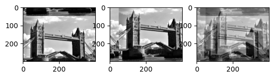
First let’s look at the library function roll:

a = np.roll(flatten, 50, axis=0)
b = np.roll(flatten, 50, axis=1)
c = a+b
imrow(a, b, c/np.amax(c))

# data parallel implementation of box filter
def simple_average(image,r):
    out = np.zeros(image.shape)
    r_ = int(r/2)
    for i in range(-r_,r_):
        for j in range(-r_,r_):
            out += np.roll(np.roll(image,i,axis=0),j,axis=1)
    return out*1.0/(r*r)

imrow(img.uniform_filter(flatten,10),simple_average(flatten,10))

We can also implement general convolutions with masks by computing a weighted average/sum.

# data parallel implementation of convolution
def simple_convolve(image, mask):
    mw, mh = mask.shape
    out = np.zeros(image.shape)
    for i in range(mw):
        for j in range(mh):
            out += mask[i, j]*np.roll(np.roll(image,
                                      int(mw/2-i), axis=0), int(mh/2-j), axis=1)
    return out

imrow(img.convolve(flatten,mask), simple_convolve(flatten,mask))